The Infinite Decay of Loyalty

When most businesses think of customers, they think of them as someones with which they have more than a fleeting engagement. It therefore makes sense to think of engagement lengths, or in other words, for how long a customer is a customer. If your business falls within this category, you are likely to have asked yourself how long an average customer engagement is. If you also have a valid answer to this question, based on your particular circumstances, then I congratulate you. As it turns out, the question “How long is an average customer engagement length?” is in almost all cases ill formulated and impossible to answer. All hope is not lost, however, as we shall see.

First, let us address the issue with the question itself. In any business over a certain size, there will be some customers that are loyal to the bone. They will stay with the business no matter what, until the demise of themselves or the business. Let us call this group the “eternals”. For the sake of illustration, even though not entirely mathematically correct, let these represent infinite engagement lengths. Now, remind yourself of how an average is calculated, as the sum of some engagement lengths divided by the number of customers having these lengths. If but one of your customers is an “eternal” the sum will be infinite, with your number of customers remaining finite, yielding an infinite average.

In reality, “eternals” stay for a very long but indefinite time, not infinitely long. Regardless, the previous discussion establishes that an average will be skewed to the point of uselessness or impossible to determine because of these customers. Interestingly, changing the question slightly circumvents the problem. If you instead ask “What is the median customer engagement length?”, it suddenly becomes much more approachable. Recall that the median is the value in the ‘middle’ of an ordered set of numbers. Given the engagement lengths 1, 8, 4, 6, 9, we order these by size to become 1, 4, 6, 8, 9, and conclude that 6 can be found in the middle and is therefore the median value. When the set of numbers has an even count, the median is the average of the two midmost numbers. The important feature of the median is that it is resilient to edge cases. Even if an infinite engagement length is added to the set, the median can still be calculated. This holds true as long as you do not have more than 50% “eternals” in your customer base.

The median engagement length represents the half life of your customer base. For a given cohort, say the customers signing up a certain year, after the median engagement length in years have passed, half of them are expected to remain. That is quite an understandable measure, but one problem still remains. In order to calculate the median, at least half of a cohort must have left. If the median engagement length is indeed years for your business, would you want to wait that long to figure it out? Of course not. Now this is a scenario I’ve found myself in more than once. With very little data, find a way to figure out the median engagement length. Surprisingly and somewhat happenstance, when I was looking for solutions, I stumbled upon what may be a universal pattern for how loyalty evolves over time. You see, most forecasting is done using curve fitting techniques, and finding the right equation is key. If you have only two or three points, there are lots of equations that you can apply, most of which will have very poor predictive power.

Fortunately, I happened to be at a company some 10 years ago where there were five yearly cohorts, whose development I could follow for 1, 2, 3, 4, and 5 years respectively. When plotting these the first year of every cohort aligned almost perfectly. That indicated to me that there is some universality in the behavior of loyalty. The surprising part was that for four of the cohorts, the first two points aligned, for three the first three, and so on. Now, this indicates that there is indeed some equation that can describe loyalty at this particular company. When found, it would with rather good accuracy predict the engagement lengths of whole cohorts, even brand new ones it seemed.

Looking at the shape of the curve the points were aligning to, it dropped off quite heavily in the first year, followed by successively smaller drops. The happenstance was that I recognized this type of curve. In a fortunate turn of events I had a couple of years earlier been working with calculations on the radioactivity of matter, and the beginning of this curve looked very much like exponential decay.

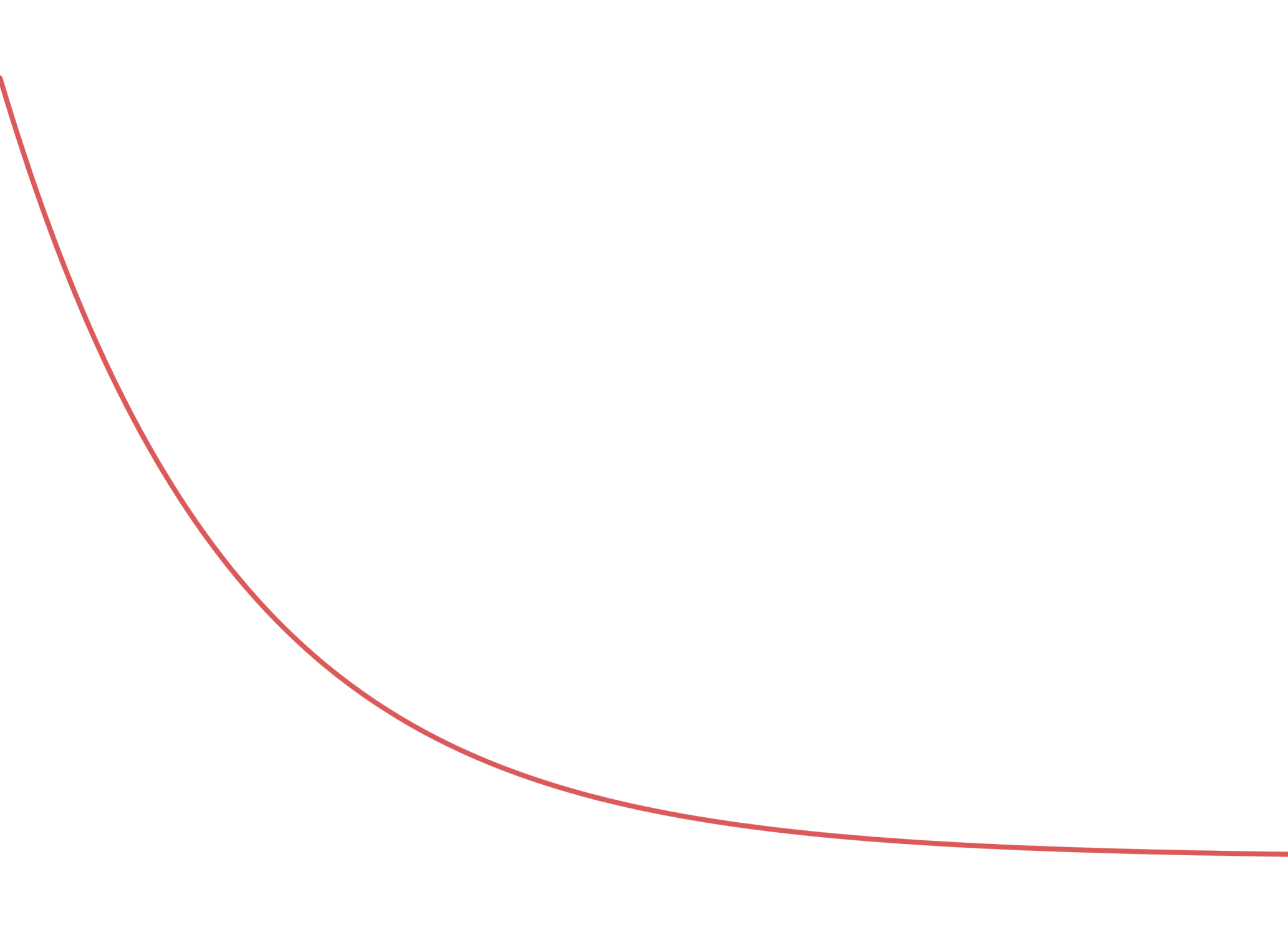
In exponential decay there is a fixed amount time that passes before a cohort is halved. If you restart there, and view this as a new cohort, after the same amount of time it will halve again. Using Excel goal seek (poor man’s brute forcing), with the formula below for exponential decay I was able to quickly figure out the half life of the cohorts I had at hand. Since the half life coincides with the median I was then able to answer the question “What is the median customer engagement length?” with some confidence, even if we had not passed that point in time yet.

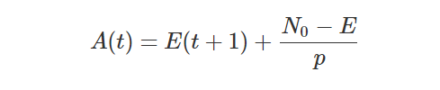
In the formula N₀ is the original cohort size, t are the points in time at which you know the actual size N(t), and h is the half life constant you need to determine. In fact, looking at it purely mathematically, it is actually possible to determine the average engagement length as well, if it were to behave exactly like exponential decay. This is, however, again under the assumption that you have no “eternals” and that your cohort will truncate to zero customers once decay has brought it down to less than the number 1. Wikipedia also notes that behavior is better understood as long as the cohort is large.

“Many decay processes that are often treated as exponential, are really only exponential so long as the sample is large and the law of large numbers holds. For small samples, a more general analysis is necessary, accounting for a Poisson process.”

Now, some will likely find it extreme to assume that loyalty is decaying exponentially. But, if we dive a bit deeper, it actually turns out to be the most natural assumption. Let us change the approach and instead think of a customer as having a fixed probability to churn during a given time frame. For example, if we are looking at monthly cohorts, let p be the probability that a customer has churned in a month. For simplicity we assume all customers have the same probability to churn, but in reality some will be more likely and others less likely. Even so, there will be an average corresponding to the actual number of customers lost around which the individual probabilities are distributed, in some fashion. After a month we would then get that (1-p) N₀ customers remain, after two months (1-p)(1-p) N₀, and so on.

This is a recursive formula that produces a series. Interestingly, if we find the correct probability this series can be made to match exponential decay perfectly.

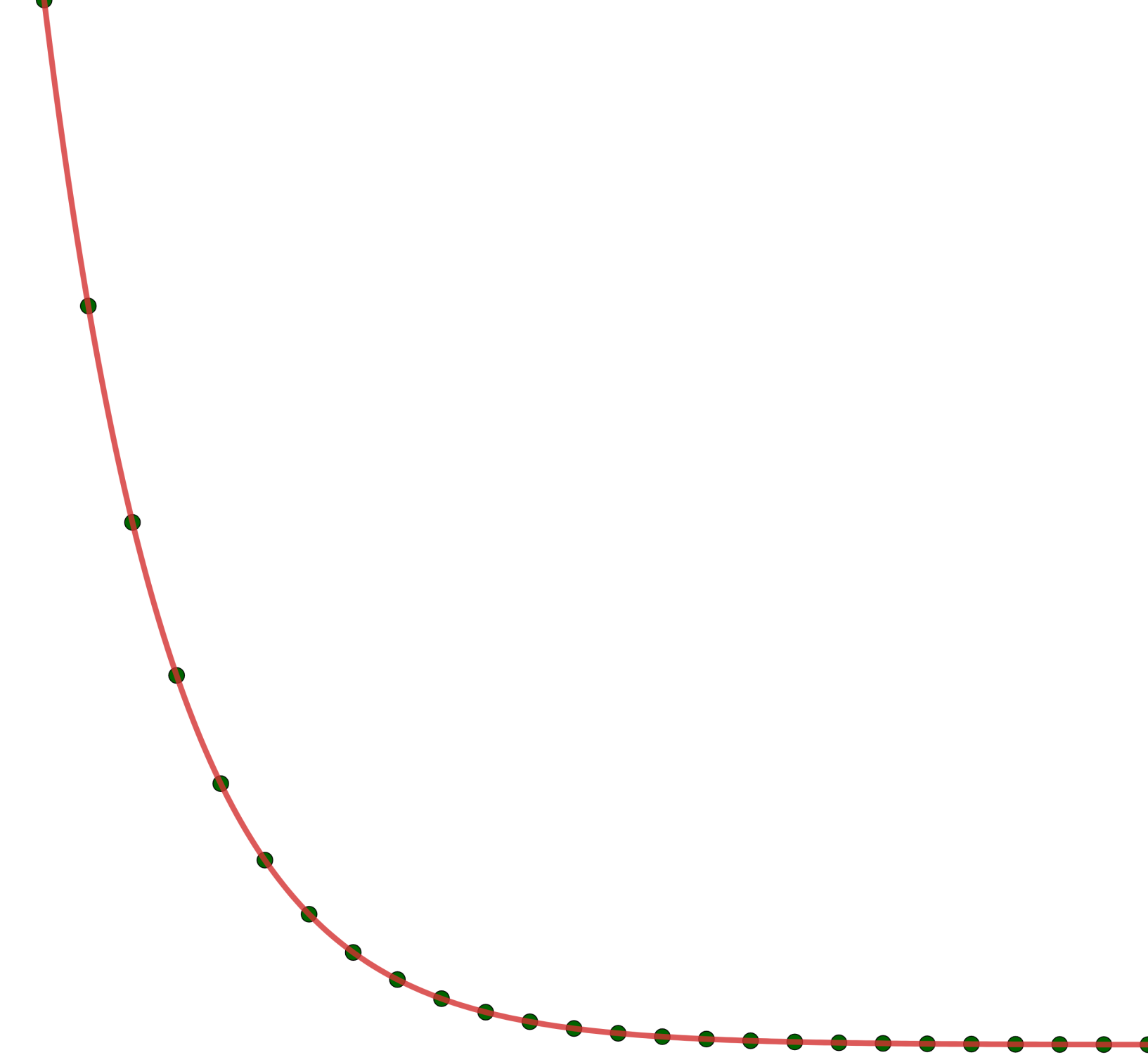
From this we can conclude that if customers have a reasonably similar probability to churn in given time frames, the end result is necessarily exponential decay. If you want to play around with this series and curve you can do so in my online workbook in GeoGebra. Given a half life h, the formula to calculate p is as follows. For example, in order to get a half life of two time periods, a churn rate of approximately 29% per period is needed.

Graphs like the one displayed by the exponential decay are called asymptotic, because as time approaches infinity the curve will approach zero. It is not hard to figure out that if the curve instead approached the number of “eternals” it would be an even better fit to the actual conditions. Changing the formula to accommodate for this is simple:

The formula is very similar to the earlier one, but now with the additional constant E, representing the number of “eternals”. Of course, this is another number not known, and the additional degree of freedom makes brute forcing their values harder, but far from impossible. The Excel Solver plugin can do multivariate goal seeks, for example.

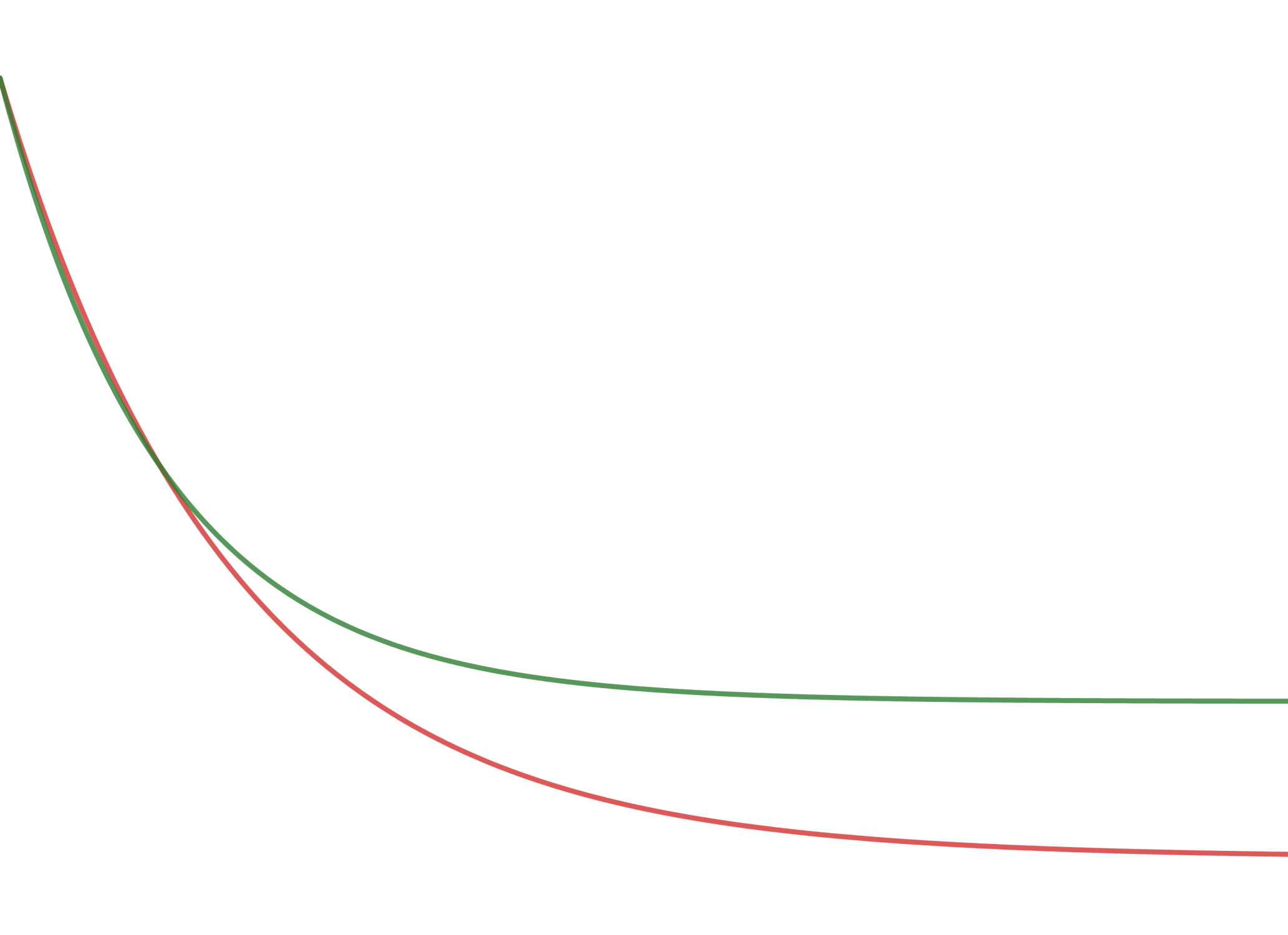
The green curve above is using the new formula, with a likely exaggerated 20% eternals. Both of these have the half life set to two time units. Given how closely these overlap before the first halving, they are likely to be inseparable when doing curve fitting early on. They do, however, diverge significantly thereafter, so determining E should become easier shortly after the first halving. Before that, estimating E must be done through other means, like actually engaging with and talking to customers, or in the worst case, through gut feelings.

Note that in the new formula the half life h pertains to the time it takes to halve the number of “non-eternals”. In order to get the new adjusted value for the constant given a desired half life, it must be multiplied by the unwieldy factor below. In the graph above the value h = 1.41504 gives an actual half life of two time units.

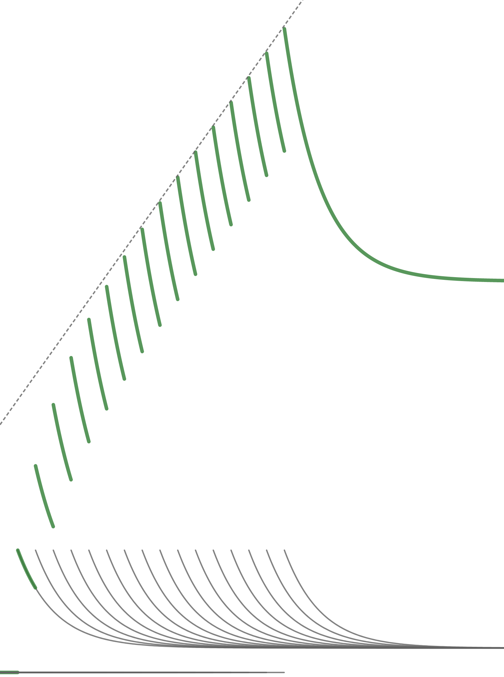
Assuming that all cohorts will behave like this, and that there is a recurring inflow of new customers, one can investigate the effects this has on a customer base over a longer period of time. If we start by taking the example of decaying cohorts without “eternals” and look at 15 consecutive time periods of acquisition, another surprise is in store for us.

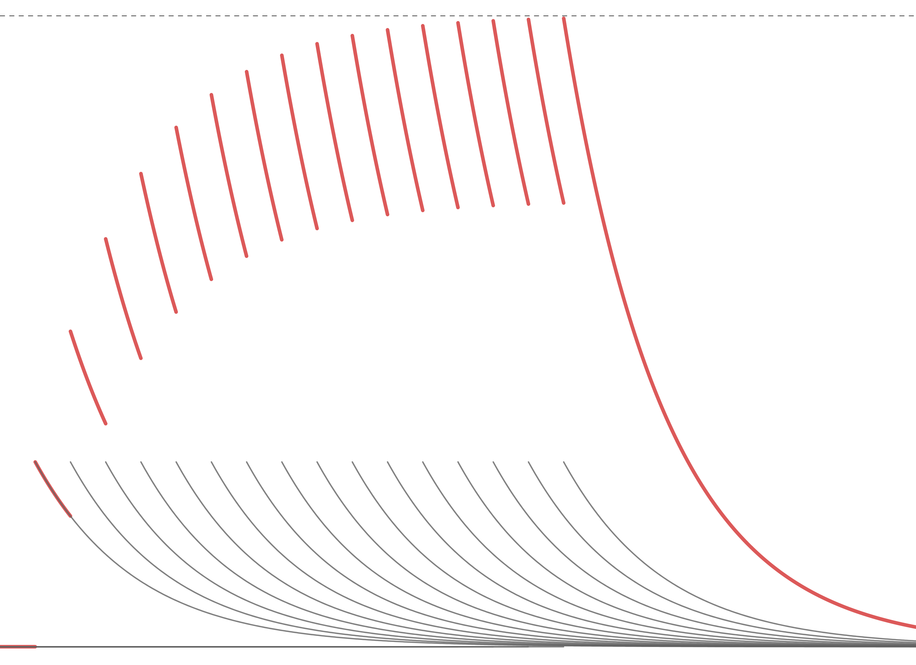
The red curve is the sum of all the individual, gray, cohort curves, so it is in effect what the total customer base will look like. In reality customers will likely not come in bursts between each time period, but somewhat more continuously. That would just reduce the jaggedness of the curve, but it would still retain its general shape. What is particularly interesting about this shape is that it is not constantly growing, even though we adding the same number of new customers every time period. The customer base grows fast in the beginning, but then the growth stalls. This is a mathematical inevitability.

With a constant inflow of new customers, an exponential decay of loyalty will eventually stall the growth of your customer base.

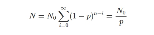
If you noticed the dotted line in the graph above it is the upper bound, the largest number of customers you will ever get. This number can actually be calculated using the ratio in the rightmost part of the formula below. With the example of a 29% churn rate per time period, the largest number of customers is between three and four times a cohort size.

Over time, some customers are bound to return after a hiatus, at which point a business may view them as new again. Returning customers, even if the business has forgotten them in the meantime, are just a variation of “eternals”. The graph above is, in other words, only valid when there are no “eternals”, neither constant nor alternating. Let us therefore look at a similar graph for the more true to life example of decaying cohorts with “eternals”.

When “eternals” are part of the equation, the growth no longer stalls, and instead becomes more or less linear after an initial phase of more rapid growth. Recall that we use the likely exaggerated 20% in these examples, which is why the line is rather steep. This is, however, an indication that even a small percentage of “eternals” will make a significant difference in the development of your customer base.

Sustained growth of a customer base is only possible when some are eternally loyal.

That being said, growth cannot continue forever for other reasons. There is a limited number of people living on this planet, or more likely a limited number of people in your target market, in which there is also competition for the customers. This places an upper limit to the possible market share any business can get. Even so, understanding the mathematical fundamentals of customer base growth and applying these to your situation can yield early and important insights.

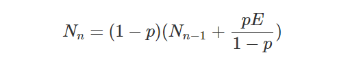
Now, let us return to the dotted line in the final graph and see if we can find its equation. First, the recursive formula will have to be adjusted for the presence of “eternals”, so that it becomes as follows.

When many such series are summed up, one for each cohort, the resulting total sum becomes the sum of the individual terms up to n.

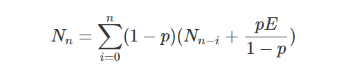
From this the equation for the linear asymptote can be determined, and that line is described by the following equation, where t is the time passed.

With all the intellectually challenging and rather complex work done, what remains is that rather simple equation, which in essence describes the long term behavior of your customer base growth. From it, you can easily see that if E = 0 we get the simpler and constant upper bond discussed earlier. We can also see that the steepness of the asymptote is independent of your churn rate, p. Halving the churn rate, for example, will not double your customer base growth. Also, the smaller your churn rate is, the less the effect will be of reducing it further.

Both increasing the number of “eternals” and reducing the churn rate suffers from diminishing returns. A small change will result in a relatively even smaller change in growth, and the more loyal your customers become, the less the effect will be.

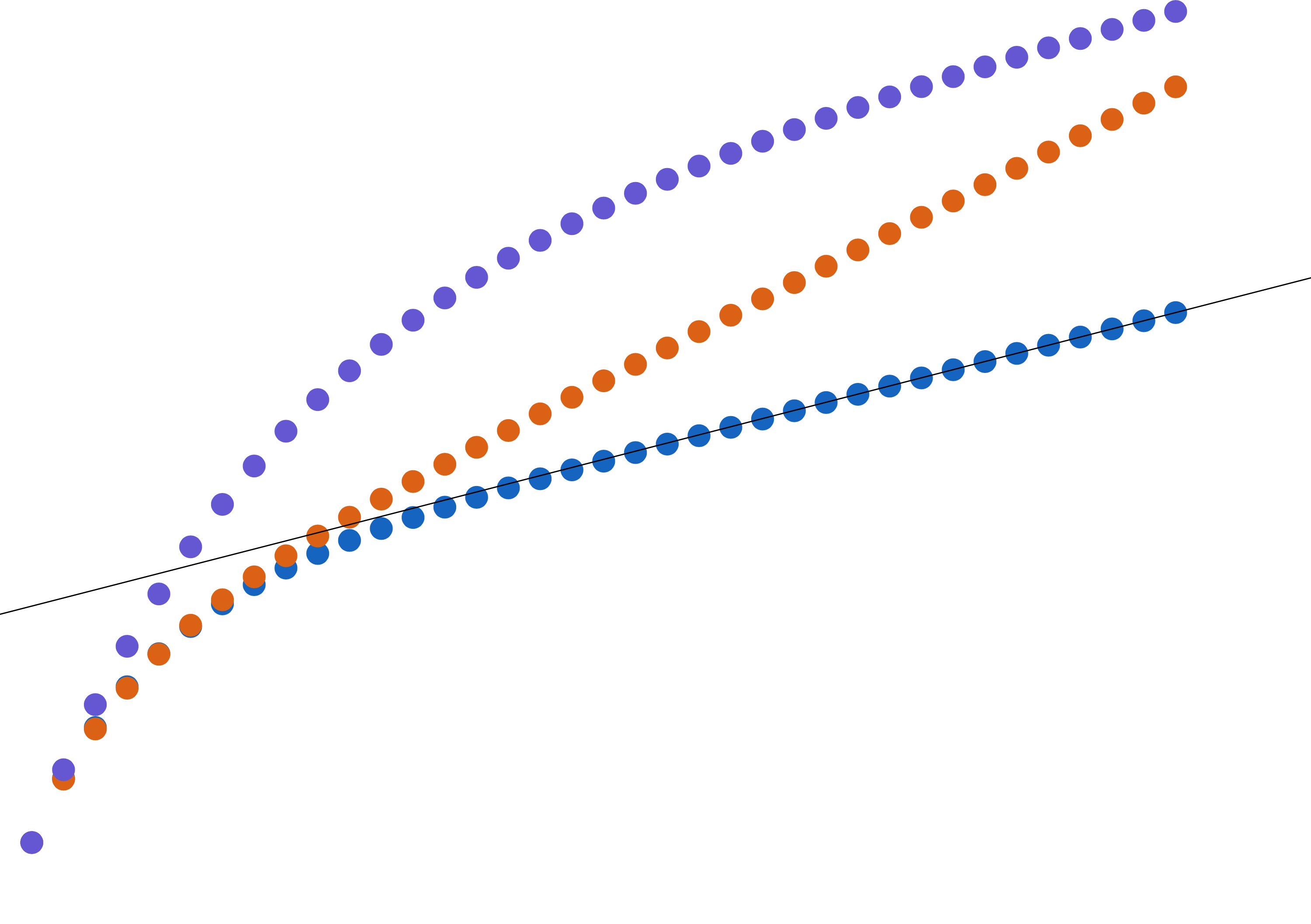
In the graph above, the purple growth is after halving the churn rate, compared to the blue growth. The orange growth is instead doubling the number of eternals. The long term effect of doubling the number of “eternals” is a higher sustained growth rate, and had the graph been longer it would soon have overtaken the halved churn rate. Efforts aimed to produce “eternals” are therefore more important than efforts to reduce general churn.

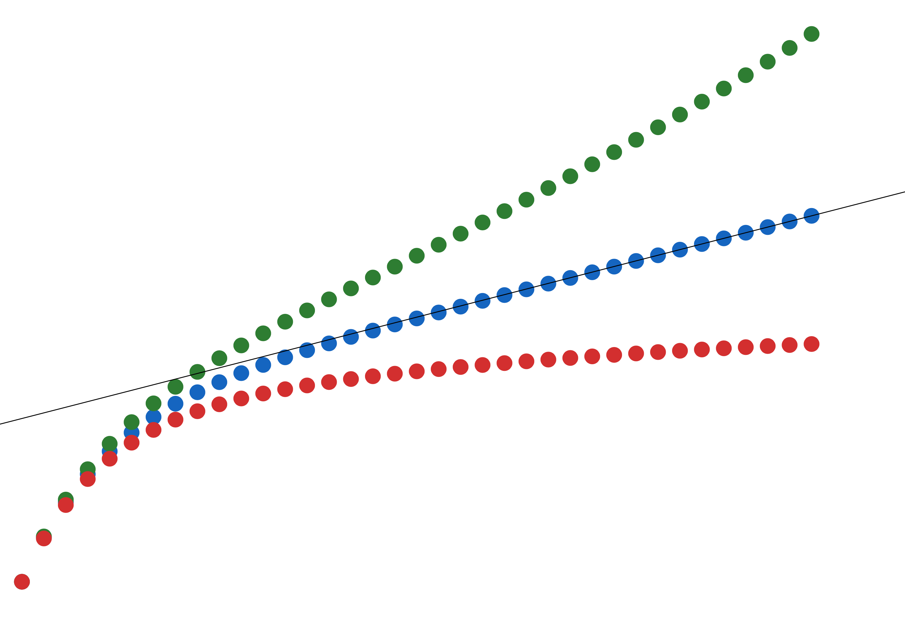
With all that said, there is still one parameter that we have not tinkered with. Everything so far has relied on the assumption that the inflow is constant, every cohort has the same size. For a mature business, this is not an unlikely scenario though. But, what if the cohorts themselves grow or shrink? How would that effect compare to the effects of increasing loyalty? In the graph below, the green growth has a 1% increase in the cohort size between every point. Similarly, the red growth has a 1% decrease in cohort size. Somewhat astoundingly, such a small increase will equal the effects of doubling the “eternals”. More frighteningly, with a small decrease, the growth will again almost completely stall. This places the importance of sales in a new perspective.

Efforts to produce incremental increase in customer inflow vastly outweigh efforts to increase loyalty in terms of effect on growth.

But, does this really apply to your business? I cannot answer that question with certainty, but I can say that in the original business where I discovered this 10 years ago, recent cohorts still adhere to this behavior, and old ones have not diverged from what was predicted. We, at the company where I work now, have also applied this at two other businesses in completely different domains and other stages of development. It was a bit of a long shot, but it turns out that the patterns holds true also for them. Loyalty is decaying exponentially. Now, this is the reason why I am writing this, because I am suspecting that this could be an innate and universal property of loyalty.

I know that most of you won’t go back and start doing calculations, but to those of you who do, please let me know the results!

If this indeed holds true, even within a limited scope, spreading this knowledge should prove valuable for many.