Atomic Data

We failed. I recently attended the Knowledge Gap conference, where we had several discussions related to data modeling. We all agreed that we are in a distressful situation both concerning the art as a whole but also its place in modern architectures, at least when it comes to integrated data models. As an art, we are seeing a decline both in interest and schooling, with practitioners shying away from its complexity and the topic disappearing from curriculums. Modern data stacks are primarily based on shuffling data and new architectures, like the data mesh, propose a decentralized organization around data, making integration an even harder task.

When I say we failed, it is because data modeling in its current form will not take off. Sure we have successful implementations and modelers with both expertise and experience in Ensemble Modeling techniques, like Anchor modeling, Data Vault and Focal. There is, however, not enough of them and as long as we are not the buzz, opportunities to actually prove that this works and works well will wane. We tried, but we’re being pushed out. We can push back, and push back harder, but I doubt we can topple the buzzwall. I won’t stop pushing, but maybe it’s also time to peek at the other side of the wall.

If we begin to accept that there will only be a select few who can build and maintain models, but many more who will push data through the stack or provide data products, is there anything we can do to embrace such a scenario?

Data Whisperers

Having given this some thought I believe I have found one big issue, preventing us from managing data in motion as well as we should. Every time we move data around we also make alterations to its representation. It’s like Chinese Whispers (aka the telephone game) in which we are lucky to retain the original message when it reaches the last recipient, given that the message is whispered from each participant to the next. A piece of information is, loosely speaking, some bundle of stuff with a possible semantic interpretation. What we are doing in almost all solutions today is to, best we can, pass on and preserve the semantic interpretation, but care less about the bundle it came in. We are all data whisperers, but in this case that’s a bad thing.

Let’s turn this around. What if we could somehow pass a bundle around without having to understand the possible semantic interpretation? In order to do that, the bundle would have to have some form that would ensure it remained unaltered by the transfer, and that defers the semantic interpretation. Furthermore, whatever is moving such bundles around cannot be surprised by their form (read like throwing an exception), so this calls for a standard. A standard we do not have. There is no widely adopted standard for messaging pieces of information, and herein lies much of the problem.

The Atoms of Data

Imagine it was possible to create atoms of data. Stable, indivisible pieces of information that can remain unchanged through transfer and duplication, and that can be put into a grander context later. The very same piece could live in a source system, or in a data product layer, or in a data pipeline, or in a data warehouse, or all of the above, looking exactly the same everywhere. Imagine there was both a storage medium and a communication protocol for such pieces. Now, let me explain how this solves many of the issues we are facing.

Let’s say you are only interested in shuffling pieces around. With atomic data pieces you are safe from mangling the message on the way. Regardless of how many times you have moved a piece around, it will have retained its original form. What could have happened in your pipelines though, is that you have dressed up your pieces with additional pieces. Adding context on the way.

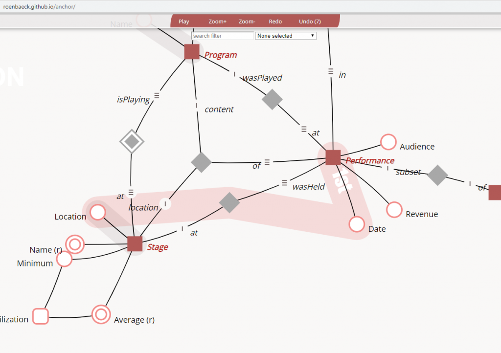
Let’s say your are building an integrated enterprise-wide model. Now you are taking lots of pieces and want to understand how these fit into an integrated data model. But, the model itself is also information, so it should be able to be described using some atoms of its own. The model becomes a part of your sea of atoms, floating alongside the pieces it describes. It is no longer a piece of paper printed from some particular modeling tool. It lives and evolves along with the rest of your data.

Let’s say you are building a data product in a data mesh. Your product will shuffle pieces to data consumers, or readers may be a better word, since pieces need not be destroyed at the receiving side. Some of them may be “bare” pieces, that have not yet been dressed up with a model, some may be dressed up with a product-local model and some may have inherited their model from an enterprise-wide model. Regardless of which, if two pieces from different products are identical, they represent the same piece of information, modeled or not.

Model More Later

Now, I have not been entirely truthful in my description of the data atoms. Passing messages around in a standardized way needs some sort of structure, and whatever that structure consists of must be agreed upon. The more universal such an agreement is, the better the interoperability and the smaller the risk of misinterpreting the message. What exactly this is, the things you have to agree upon, is also a model of sorts. In other words, no messaging without at least some kind of model.

We like to model. Perhaps we even like to model a little bit too much. Let us try to forget about what we know about modeling for a little while, and instead try to find the smallest number of things we have to agree upon in order to pass a message. What, similar to a regular atom, are the elementary particles that data atoms consist of? If we can find this set of requirements and it proves to be smaller than what we usually think of when it comes to modeling, then perhaps we can model a little first and model more later.

Model Little First

As it happens, minimal modeling has been my primary interest and topic of research for the last few years. Those interested in a deeper dive can read up on transitional modeling, in which atomic data pieces are explored in detail. In essence, the whole theory rests upon a single structure; the posit.

posit_thing [{(X_thing, role_1), ..., (Y_thing, role_n)}, value, time]

The posit acts as an atomic piece of data, so we will use it to illustrate the concept. It consists of some elements put together, for which it is desired to have a universal agreement, at least within the scope in which your data will be used.

  • There is one or more things, like X_thing and Y_thing, and the posit itself is a thing.
  • Each thing takes on a role, like role_1 to role_n, indicating how these things appear.
  • There is a value, which is what appears for the things taking on these roles.
  • There is a time, which is when this value is appearing.

Things, roles, values, and times are the elements of a posit, like elementary particles build up an atom. Of these, roles need modeling and less commonly, if values or times can be of complex types, they may also need modeling. If we focus on the roles, they will provide a vocabulary, and it is through these posits later gain interpretability and relatability to real events.

p01 [{(Archie, beard color)}, "red", '2001-01-01']
p02 [{(Archie, husband), (Bella, wife)}, "married", '2004-06-19']

The two posits above could be interpreted as:

  • When Archie is seen through the beard color role, the value “red” appears since ‘2001-01-01’.
  • When Archie is seen through the husband role and Bella through the wife role, the value “married” appears since ‘2004-06-19’.

Noteworthy here is that both what we traditionally separate into properties and relationships is managed by the same structure. Relationships in transitional modeling are also properties, but that take several things in order to appear.

Now, the little modeling that has to be done, agreeing upon which roles to use is surely not an insurmountable task. A vocabulary of roles is also easy to document, communicate and adhere to. Then, with the little modeling out of the way, we’re on to the grander things again.

Decoupling Classification

Most modeling techniques, at least current ones, begin with entities. Having figured out the entities, a model describing them and their connections is made, and only after this model is rigidly put into database, things are added. This is where atomic data turns things upside down. With atomic data, lots of things can be added to a database first, then at some later point in time, these can be dressed up with more context, like an entity-model. The dressing up can also be left to a much smaller number of people if desired (like integration modeling experts).

p03 [{(Archie, thing), (Person, class)}, "classified", '1989-08-20']

After a while I realize that I have a lot of things in the database that may have a beard color and get married, so I decide to classify these as Persons. Sometime later I also need to keep track of Golf Players.

p04 [{Archie, thing), (Golf Player, class)}, "classified", '2010-07-01']

No problem here. Multiple classifications can co-exist. Maybe Archie at some point also stops playing golf.

p05 [{(Archie, thing), (Golf Player, class)}, "declassified", '2022-06-08']

Again, not a problem. Classification does not have to be static. While a single long-lasting classification is desirable, I believe we have put too much emphasis on static entity-models. Loosening up classification, so that a thing can actually be seen as more than one type of entity and that classifications can expire over time will allow for models being very specific, yield much more flexibility and extend the longevity of kept data far beyond what we have seen so far. Remember that our atomic pieces are unchanged and remain, regardless of what we do with their classifications.

Multitenancy

Two departments in your organization are developing their own data products. Let us also assume that in this example it makes sense for one department to view Archie as a Person and for the other to view Archie as a Golf Player. We will call the Person department “financial” and it additionally needs to keep track of Archie’s account number. We will call the Golf Player department “member” and it additionally needs to keep track of Archie’s golf handicap. First, the posits for the account number and golf handicap are:

p06 [{(Archie, account number)}, 555-12345-42, '2018-01-01']
p07 [{(Archie, golf handicap)}, 36, '2022-05-18']

These posits may live their entire lives in the different data products and never reside together, or they could be copied to temporarily live together for a particular analysis, or they could permanently be stored right next to each other in an integrated database. It does not matter. The original and any copies will remain identical. With those in place, it’s time to add information about the way each department view these.

p08 [{(p03, posit), (Financial Dept, ascertains)}, 100%, '2019-12-31']
p09 [{(p04, posit), (Member Dept, ascertains)}, 100%, '2020-01-01']
p10 [{(p06, posit), (Financial Dept, ascertains)}, 100%, '2019-12-31']
p11 [{(p07, posit), (Member Dept, ascertains)}, 75%, '2020-01-01']

The posits above are called assertions, and they are metadata, since they talk about other posits. Information about information. An assertion records someone’s opinion of a posit and the value that appears is the certainty of that opinion. In the case of 100%, this corresponds to absolute certainty that whatever the posit is stating is true. The Member Department is less certain about the handicap, perhaps because the source of the data is less reliable.

Using assertions, it is possible to keep track of who thinks what in the organization. It also makes it possible to have different models for different parts of the organization. In an enterprise wide integrated model, perhaps both classifications are asserted by the Enterprise Dept, or some completely different classification is used. You have the freedom to do whatever you want.

Immutability

Atomic data only works well if the data atoms remain unchanged. You would not want to end up in a situation where a copy of a posit stored elsewhere than the original all of a sudden looks different from it. Data atoms, the posits, need to be immutable. But, we live in a world where everything is changing, all the time, and we are not infallible, so mistakes can be made.

While managing change and immutability may sound like incompatible requirements, it is possible to have both, thanks to the time in the posit and through assertions. Depending on if what you are facing is a new version or a correction it is handled differently. If the beard of Archie turns gray, this is a new version of his beard color. Recalling the posit about its original color and this new information gives us the following posits:

p01 [{(Archie, beard color)}, "red", '2001-01-01']
p12 [{(Archie, beard color)}, "gray", '2012-12-12']

Comparing the two posits, a version (or natural change), occurs when they have the same things and roles, but a different value at a different time. On the other hand, if someone made a mistake entering Archie’s account number, this needs to be corrected once discovered. Let’s recall the posit with the account number and the Financial Dept’s opinion, then add new posits to handle the correction.

p06 [{(Archie, account number)}, 555-12345-42, '2018-01-01']
p10 [{(p06, posit), (Financial Dept, ascertains)}, 100%, '2019-12-31']
p13 [{(p06, posit), (Financial Dept, ascertains)}, 0%, '2022-06-08']
p14 [{(Archie, account number)}, 911-12345-42, '2018-01-01']
p15 [{(p14, posit), (Financial Dept, ascertains)}, 100%, '2022-06-08']

This operation is more complicated, as it needs three new posits. First, the Financial Dept retracts its opinion about the original account number by changing its opinion to 0% certainty; complete uncertainty. For those familiar with bitemporal data, this is sometimes there referred to as a ‘logical delete’. Then a new posit is added with the correct account number, and this new posit is asserted with 100% certainty in the final posit.

Immutability takes a little bit of work, but it is necessary. Atoms cannot change their composition without becoming something else. And, as soon as something becomes something else, we are back to whispering data and inconsistencies will abound in the organization.

What’s the catch?

All of this looks absolutely great at first glance. Posits can be created anywhere in the organization provided that everyone is following the same vocabulary for the roles, after which these posits can be copied, sent around, stored, classified, dressed up with additional context, opinionated, and so on. There is, however, one catch.

Identifiers.

In the examples above we have used Archie as an identifier for some particular thing. This identifier needs to have been created somewhere. This somewhere is what owns the process of creating other things like Archie. Unless this is centralized or strictly coordinated, posits about Archie and Archie-likes cannot be created in different places. There should be a universal agreement on what thing Archie represents and no other thing may be Archie than this thing.

More likely, Archie would be stated through some kind of UID, an organizationally unique identifier. Less readable, but more likely the actual case would be:

p01 [{(9799fcf4-a47a-41b5-2d800605e695, beard color)}, "red", '2001-01-01']

The requirement for the identifier of the posit itself, p01, is less demanding. A posit depends on each of its elements, so if just one bit of a posit changes, it is a different posit. The implication of this is that identifiers for posits need not be universally agreed upon, since they can be resolved within a body of information and recreated at will. Some work has to be done when reconciling posits from several sources though. We likely do not want to centralize the process of assigning identities to posits, since that would mean communicating every posit from every system to some central authority, more or less defeating the purpose of decentralization.

Conclusions

If we are to pull off something like the data mesh, there are several key features we need to have:

  • Atomic data that can be passed around, copied, and stored without alteration.
  • As few things as possible that need to be universally agreed upon.
  • Model little first model more later, dress up data differently by locality or time.
  • Immutability so that data remains consistent across the organization.
  • Versions and corrections, while still adhering to immutability.
  • Centralized management for the assignment of identifiers.

As we have seen, getting all of these requires carefully designed data structures, like the posit, and a sound theory of how to apply them. With the work I have done, I believe we have both. What is still missing are the two things I asked you to imagine earlier, a storage medium and a communication protocol. I am well on the way to produce a storage medium in the form of the bareclad database engine, and a communication protocol should not be that difficult, given that we already have a syntax for expressing posits, as in the examples above.

If you, like me, think this is the way forward, please consider helping out in any way you can. The goal is to keep everything open and free, so if you get involved, expect it to be for the greater good. Get in touch!

We may have failed. But all is definitely not lost.

Peridata between Data and Metadata

Somewhere in between data and metadata there is another kind of information, which we will name peridata. Perhaps you have found yourself looking at some piece of information and thinking, is this data or metadata? In this article, not only will you get a precise definition of what is what, but also a term for data living on the fringe of its classification. In order to achieve these definitions, we will turn to the posit, which is the fundamental building block of transitional modeling.

Posits

A posit essentially captures a piece of information. Here are two examples:

p1 = [{(Archie, beard)}, fluffy red, 2020-01-01]
p2 = [{(Archie, husband), (Bella, wife)}, married, 2004-06-19]

The first posit, p1, captures the information that Archie had a fluffy red beard on the 1st of January 2020. The second posit, p2, captures the information that Archie and Bella are married since the 19th of June 2004. Posits can express properties, as in p1, and relationships, as in p2. In transitional modeling, relationships are properties that require more than one thing to take on a value. Such an approach may be unfamiliar, since in most other modeling techniques there are separate constructs for properties and relationships. The proper way to read those two posits, using the notion of roles, is:

When Archie filled the beard role the value ‘fluffy red‘ appeared on 2020-01-01.

When Archie filled the husband role and Bella the wife role the value ‘married‘ appeared on 2004-06-19.

A singular thing filling a singular role gives rise to what we usually call properties or attributes, whereas a combination of things filling a combination of roles give rise to relationships. Whenever roles are filled, some value appears. In the case of Bella and Archie it could just as well have been ‘divorced’, ‘planned’, or ‘not applicable’. In fact, for the vast majority of people we could fill the roles with the relationship is ‘not applicable’, but we tend to document these only in the rare cases such posits carry valuable information.

Given the terminology of things (Archie, Bellla) and roles (beard, husband, wife), the structure of a posit can be formalized as:

posit = [
  {(thing 1, role 1), ..., (thing n, role n)},
  appearing value, 
  time of appearance
]

The set in the first position of the posit is called an appearance set, followed by the for that set appearing value and its time of appearance. Posits are just pieces of information and there is no requirement that they must be true. After all, there is a lot of untrue information out there and much more, maybe even most, that is uncertain to some degree. We do not want to disqualify any information from being recorded based on its certainty.

Data and Metadata

We will now make the distinction between data and metadata. Given an appearance set, if all the things it contains are not posits, then posits containing that set are classified as data. Correspondingly, given an appearance set, if at least one of the things it contains is a posit, then posits containing the set are classified as metadata. The examples given so far are data, since neither Archie nor Bella is a posit. Instead, one of the most important examples of metadata in transitional modeling is:

p3 = [{(p1, posit), (Bella, ascertains)}, 1.00, 2020-01-02]

There is no way to determine its truthfulness from a posit alone, so an additional construct is needed. An assertion is a posit that assigns a certainty to another posit. In the example above, Bella ascertains the posit about Archie’s beard, with absolute certainty on the 2nd of January 2020. This is metadata, since p1 is a posit. Assertions are subjective, and so far we only have Bella’s view of p1. Certainty is expressed by a real number in the interval [-1, 1], where 1 is being absolutely certain of what the posit is stating, 0 is having no idea whatsoever, and -1 being certain of the opposite of what the posit is stating. If you want to delve deeper into the expressiveness given by this machinery, you can read the paper “Modeling Conflicting, Unreliable, and Varying Information“.

Another common type of metadata, particularly in data warehouses, has to do with from which source posits originated.

p4 = [{(p3, source)}, The Horse's Mouth, 2020-01-01]

There could be a whole range of information related to the posit itself, like who or what recorded it, when it was entered into a database, its associated security or sensitivity, effective constraints at the time, or rules to apply in certain scenarios. These are just some examples, but all of which would be classified as metadata, because they involve a posit in their appearance sets.

Since metadata is also expressed using posits, these can be parts of appearance sets as well. For example, in p4 the assertion p3 is a part of its appearance set, so p4 is also metadata, but on a different “level” than the already metadata p3. In such a case it makes sense to distinguish these as level-1 metadata and level-2 metadata, which could be extended up to any level-n metadata. I believe that going beyond level-1 metadata is unusual in existing implementations, and that there may be few use cases that need additional levels. However, when they are needed, they are probably also very important.

Peridata

While the rules separating data and metadata are clear cut, the way to tell data from peridata is less straightforward. In transitional modeling it is possible to reserve roles for particular purposes. One such example is used for classification.

p5 = [{(Archie, thing), (Person, class)}, active, 1972-08-20]

This posit tells us that Archie belongs to the Person class since 1972-08-20, using the reserved class role. Thanks to classification being expressed through posits, it is possible to disagree on these using assertions. It is also possible to have multiple classifications at once and to let classifications expire or become active at different points in time.

As you can see, there is no posit in the appearance set of p5, so it is not metadata by our previous definition. Although, the model is likely something that traditionally would have been classified as metadata. In order to distinguish this type of data from regular data, we will use the concept of reserved roles. But then, what are reserved roles? Well, you can think of them as being similar to reserved keywords in a programming language. In fact, in the examples so far, the roles positascertainsthing, and class are already reserved in transitional modeling. The roles beardhusband, and wife depend on your domain and are instead something you as a modeler will have to bring into existance.

With this we can get definitions for all three categories.

  1. If at least one of the things contained in an appearance set is a posit, then all posits with this set are classified as metadata.
  2. If at least one of the roles contained in an appearance set is reserved, then all posits with this set are classified as peridata.
  3. If neither of above applies to an appearance set, then all posits with such sets are classified as data.

Peridata exists among your data, but sort of on the fringe, given that it requires these reserved roles. Note that it is possible to have peridata for your metadata as well, when both 1 and 2 apply. Transitional modeling will come with a set of reserved roles, all of which are domain independent, but there will also be an option for end users to reserve roles of their own.

Remarks

Thanks to transitional modeling, we have been able to break down what is traditionally thought of as a single metadata concept into two categories, metadata and peridata. On the fringe of your data you will find peridata, short for peripheral data, which capture such things as the classifications in your domain. Metadata is restricted to those pieces of information that explicitly talk about other pieces of information. Whether this distinction is useful remains to be seen, but it is certainly interesting. In a relational database, for example, the classifications in the modeled domain exists as a schema. Schemas are therefore peridata. Perhaps you can think of other commonly used model artifacts that fall within the scope of peridata or metadata?

On a side note, there are already some indications that the use of reserved roles can improve performance in a database engine based on posits. If you are interested in following the developement of such an engine, check out bareclad.

Time in Databases

Is something in your database dependent on time? If you think not, think again. I can assure you there are plenty of such things. But, as plentiful as your time-dependent objects are, as plentiful are the creative ways I’ve seen them handled. Trust me, when you screw up time, the failures of your implementation will be felt, painfully. This is, however, understandable given the complexity of time and its limited treatment in commonplace database literature. This article aims to introduce a terminology together with some best practices and considerations that should be addressed before implementing time in a database. It is inspired by the article “Kinds of Time” by Christian Kaul, and likely has significant overlaps, but provides my slightly different view.

Primary and Documentary Times

In essence there are two purposes time can serve in a database. Time can be of a primary nature or of a documentary nature. Time of a primary nature is part of your primary keys, and your database engine will, if modeled accordingly, automatically ensure temporal integrity with respect to it. Time of a documentary nature are data points that are of a time type, like a date, but that are not part of your primary keys. If you need any constraints imposed over your documentary time, you will have to build and maintain them yourself.

For integrity reasons, any primary time values must be comparable in such a way that they form a total order. Time of day, such as 12:59, cannot be used as it will repeat itself daily, giving you no option to determine if two instances of 12:59 coincided or happened in some succession. Because of this requirement, primary times are often expressed through some calendar convention, such as Julian day, Unix time, or perhaps most commonly ISO 8601, which even accommodates for leap seconds. It is worth noting that any time that is affected by daylight saving is not totally ordered. In Sweden the hour between 02:00 and 03:00 on the last Sunday of October is repeated every year. Even so and unfortunately, I see many databases here use local time as primary time.

A decent choice for a primary time would therefore be coordinated universal time (UTC). Expressed in ISO 8601, such a time looks like 2021-01-25T07:23:47.534Z. While this may look satisfactory, there is an additional concern. The precision of the data type used to store this time in the database may debilitate the total ordering. Somewhat surprisingly, and often nastily discovered, the precision of a datetime in SQL Server is 3 milliseconds. The final digit in a time expressed as above can only be 0, 3 or 7 in the database. While this particular choice is unintuitive, there is always a shortest time span that can be represented through a data type, called its chronon. For primary times, a data type with a chronon shorter than anything happening in succession is necessary to preserve the total ordering.

Given that primary times are parts of primary keys in the database and altering primary keys is normally time-consuming, the choice of data types should be made with care. Always picking the data type with the smallest chronon, such as datetime2(7) in SQL Server with a 100 nanosecond chronon, may affect performance. While it can store a time like 2007-05-02T19:58:47.1234567 it will use 8 bytes, compared to 3 bytes for the date type, if daily changes are sufficient. Keeping primary keys small should be paramount for any database designer, since smaller keys lowers total storage and increase insert and join performance.

Documentary times are not required to have a total ordering or even be temporally consistent, making it possible for versions overlapping in time. With so much leniency choices can be made with much less consideration. Naturally, there are cases when you want to impose the same restrictions to documentary times, particularly if you intend for them to behave as primary times at some point.

Particular Recurring Timepoints

There are some particular recurring timepoints of interest, and for some reason beyond my understanding there is no standardised way to express these. Some common ones are:

  • The end of time.
  • The beginning of time.
  • Indefinitely.
  • At an unknown time.

The end of time is what it sounds like, the infinite extension of time into the future. An application for this would be if you want to express a fact such as ‘I will love you forever’. Similarly, the beginning of time is the longest possible extension of time into the past. It could be applied in an expression such as ‘gravity has always been present in the universe’. Indefinitely is similar to these, but in this case we expect an actual point in time will come to pass after which a time interval is no longer open-ended. An application, with the slight but important difference from ‘forever’ is ‘I will cherish rock music until the day I die’ or ‘my hair will turn gray one day’. Finally, there is the unknown time. It can be used both for past and future events, such as ‘The price was raised, but nobody remembers when that happened’ and ‘We will raise the price the next time crops fail’.

From a storage perspective, databases normally provide one special value; NULL, that is (somewhat horrifyingly) often used for all purposes above. Practically one could possibly reason that unknown time could be used in place of indefinitely, which in turn could be used in place of the beginning and end of time. Semantically, some important nuances will then be lost. For example, the nuance lost by stating ‘I will love you until an unknown time’ may yield an entirely different outcome.

Ideally, and if your database permits user-defined types, data types which includes and separates these particular timepoints should be implemented. ISO 8601 should also be extended with ways to express these notions. There is an interesting discussion on how to express these by shema.org here, for anyone who wants to dive deeper, which suggests that standards may be coming. Regardless, you should consider how you intend to manage particular timepoints like these.

Named Timelines

Even if there is just one single time, there are many timelines. A timeline can be thought of as an interval of time (finite or infinite) over which events happen in a temporally consistent sequence. If two events can mess up each others bonds in time, such as one moving the other in time, then they definitely do not belong on the same timeline. For example, if I have an appointment in my calendar between 9:00 and 10:00 today it lives on a different timeline from the action of me, at 08:00, rescheduling it to the afternoon. Timelines can also be separated by the fact that the events they track pertain to completely different things, and it would only decrease readability and understandability to keep them together.

Borrowing the terminology of transitional modeling, following are some examples of timelines commonly discussed in computer science and database literature. There is so little consensus on the naming of these so understanding what they represent is what matters.

The Appearance Timeline

The appearance timeline contain points in time when some value was observed, became valid, or will come into effect in real life. It tracks the natural progression between values or states, both for attributes and relationships. Note that appearance timepoints may lie in the future, such as an already known price cut coming into effect on Black Friday.

In literature it is known by many different names: Valid time [Snodgrass], Effective time [Johnston], Application time [ANSI SQL:2011], and Changing time [Anchor modeling]. I also recall hearing these synonyms from forgotten sources: Utterance time, State time, Business time, Versioning time, and Statement time.

The Assertion Timeline

The assertion timeline contains points in time when some statement is subjectively assessed with respect to its certainty. In the simple case this is done by some system acting as the asserter and statements evaluating to either true or false. It is commonly used to track the correction or deletion of values or states, both for attributes and relationships. Note that assertion timepoints cannot lie in the future. If someone corrects the rebate for the upcoming price cut on Black Friday, this correction necessarily happens in the present.

In literature it is also known by many different names: Transaction time [Snodgrass], Assertion time [Johnston], System versioning time [ANSI SQL:2011], and Positing time [Anchor modeling]. I have heard less synonyms here from forgotten sources, only Falsification time and Evaluation time comes to mind.

For further reading on how to make uncertain assertions, to even being sure of the opposite, there is more information on transitional modeling in this series of articles.

The Recording Timeline

The recording timeline contains points in time at which information is stored in some kind of memory, typically when the data entered the database. This is very useful from a logging and later maintenance perspective. With it you can keep track of how quickly your database is growing on a per object basis, or revert to previous states of the database, perhaps after an erroneous load. It could have been the case that I sent all the price cuts for Black Friday into the production database but associated with the wrong products due to a faulty join.

In literature there are a couple of other names: Inscription time [Johnston] and Load date [Data Vault]. A very poor synonym I’ve seen used is Transaction time, which should be reserved for the assertion timeline alone.

The Structuring Timeline

The structuring timeline contains the point in time at which the information had a certain structure and constraints. Yes, structure and constraints change over time too. This process is referred to as schema versioning in literature, but few mention keeping a named time line for tracking when structural changes happened. If someone comes asking why there were no price cuts for Black Friday last year, you can safely assure them that ‘price cut’ was not part of your information structure at the time.

The only other name I have seen is Schema Versioning Time, but it has a too technical ring to it, in my opinion.

Unnamed Timelines

Unnamed timelines are all the points in time that do not fall within any of your named timelines. There will be values in your database that are of a time type, but that are not immediately put onto named timelines, even if the attributes themselves are named. These may be assembled onto timelines for ad-hoc purposes or they may just be used as any other descriptive attribute. A typical example would be the point of time the receipt for the stuff I bought on Black Friday was printed. You are not likely to name the timeline on which birth dates occur either.

In literature there are a couple of other names: User defined time [Snodgrass] and Happening time [Anchor]. Again, I’ve seen Transaction time used for unnamed times when the timepoint represents some event in which a transaction took place. Again, an unfortunate confusion of terminology.

Time Tracking Scope

Before implementing time in your database, you need to consider which of the timelines above and possibly others you will need, since they need to be separable in your database, possibly as different columns in the same or adjoined tables. Along with that you will also need to determine your time tracking scope. For example, is it sufficient to track changes to any part of an address or do you need to track changes of the individual parts of an address?

If tracking any change is sufficient, you can use a single point in time for the entire address. Essentially, you will be viewing a changed address, regardless of which part changed, as a new address. If you track the individual parts you will need several points in time, one for the street, one for the postal code, one for the state, and so on. In this case the same address can have different postal codes over time.

The latter approach, tracking time for every single object (attribute and relationship) can be achieved through modeling in the sixth normal form, henceforth 6NF. With it change is visible without having to make comparisons with previous rows and no data is duplicated when only a part of something is changing.

Even if you do not go as far as 6NF your time tracking scope has to be decided, since the amount of timepoints you will store depend on it. Unfortunately, in many of the source systems I regularly fetch data from, there is usually just one column named “modified date” which is documentary. In other words you can only tell something has changed and when, but not exactly what or what came before it. In these situations you can, with a proper data warehouse, provide the history the sources lost.

Orthogonality

If you have an implementation that keeps track of both appearance and assertion timepoints, this is usually referred to as a bi-temporal implementation. The reason is that events on the appearance timeline are in a sense orthogonal to events on the assertion timeline. It is possible for the same value to appear and to be asserted simultaneously, but also at different times, so a single timepoint is not sufficient to describe both events. Furthermore, what value appears may be retroactively corrected by a later assertion. When a value appears may be also modified by an assertion. Keeping both of these on the same timeline, if you think of it as storing the date and time in a single column in a table, would cause collisions and ambiguities.

When appearances and assertions are easy to tell apart, using two different timepoints to describe these may be complex but straightforward. Problems usually arise when you are faced with a different value but nobody can tell whether it is a correction of the existing value or supposed to replace it from some point in time. This may lead to corrupt data if the wrong assumptions are made. Another issue is the fact that if you want a bi-temporal implementation with both appearance and assertion timelines treated as primary, a single table with a single primary key cannot guarantee temporal integrity. This requires careful modeling, and only a few modeling techniques have this as a “built-in” feature.

Proxying

Some of the most confusing aspects of time in databases come from the use of proxying, whether deliberate or unknowingly. If we assume that I have decided to keep track of appearance, assertion, recording, and structuring timelines in my database, with 6NF time tracking scope, then I am very much all set for anything thrown at me from a querying perspective. However, that is under the assumption that all of those timepoints will be available to me when I put data into my database.

Sadly, this is often not the case. This is true both for operational systems and data warehouses. Getting information like [Using the Megastore structure as of January 5th (The database recorded on Monday 10:12:42 that ‘The manager asserted with 95% certainty on Monday at 09:15 that “The price cut will be 25% starting at midnight on Black Friday”‘)], actually never happens, yet. We do get some of the information some of the time though.

If we are in control of the database, we will always know when data is entering it. This opens up an opportunity. In the case that we do not know the assertion timepoint, say we only get “The price cut will be 25% starting at midnight on Black Friday”, we can approximate it with the recording timepoint. In this example that means missing the mark by almost an hour. As unfortunate as this is, sometimes it is the only option.

Somewhat more dangerous, but also doable, is approximating appearance timepoints with recording timepoints. Let’s say we only get “The price cut will be 25%” and we approximate it with the recording timepoint we will be dropping the price several days too early. Since recording timepoints always “happen” in the present when they come into existence, take utmost care when using it as an approximation for appearance timepoints. Still, this may sometimes also be the only option available.

Here within lies the big fallacy though. When enough approximations have been done, the different timelines become hard to distinguish, and it seems like you can use these timepoints interchangeably. This is not the case. You should always strive to get hold of the times when they are available and if proxying is necessary, and only as a last resort, then structure your loading intervals accordingly, to minimise the damage done.

Comparing Data Vault and Anchor

So far we have talked about time in databases from a theoretical perspective. There are two modeling techniques I would like to take a practical look at, taking diametrically different approaches to which timelines serve what purposes. The two techniques Anchor modeling and Data Vault are related, both being forms of Ensemble modeling, but still have many differences.

Anchor modeling utilises 6NF to provide as granular time tracking scope as possible. It designates the appearance and assertion timelines as primary for both attributes and relationships (called ties) around a concept (called anchor), while the recording timeline is documentary. Ties are attribute-like since they have a primary timeline and in that they have no identity of their own, making tie-to-tie and tie-to-attribute connections impossible, and tie-to-anchors the only option. Anchor also maintains separate metadata for the information structure in which structuring time is primary. By treating appearance and assertion timelines as primary, the database engine will ensure bi-temporal integrity. However, that needs both to be present and have functionally adequate approximations when necessary. Anchor also makes the assumption that values are exhaustive, such that an existing value cannot become NULL, and must instead be explicitly marked as “Unknown”. There no NULL values in an Anchor model.

Data Vault is similar to Anchor, but is not 6NF and instead groups attributes together (called satellites) around a concept (called hub). A single point of time is used to track all changes within a satellite, regardless of which particular attribute changed. The big difference is that Data Vault uses the recording timeline as primary for satellites. Relationships (called links) have no primary, but include a recording timepoint as documentary. Links are hub-like since they lack a primary, and can therefore have their own identities. Theoretically link-to-link and link-to-satellite connections then become possible. The implication is that relationships that change over time must be managed through other connected objects. Figuring out that some change occurred requires you to look outside of the link. Links are also, opposed to ties, always many to many, so any additional constraints have to be managed by the application layer. If appearance and assertion timelines are present in satellites or elsewhere pertain to links, they are always documentary. I do not believe Data Vault has a notion of a structuring timeline in its standard.

The advantage of Anchor is that you do not have to worry about temporal integrity after the data has entered the database. Integrity is also practically a requirement if you want to use the technique outside of data warehousing. Anchor was designed to be a general modeling technique and it is applied in several operational systems. The downside is that you need trustworthy timepoints, which can require a lot of effort and digging in the sources. Values in a source that once existed and suddenly are NULL could pose a problem if they are indeed suddenly “Unknown” and your data type does not support it to be explicitly specified. This has, in my experience, very rarely happened, and almost always the NULL means ‘deleted’, as in asserting the statement as false, which is a different thing and handled without problems. Analysts find it easy to work directly with Anchor models, thanks to it being able to serve data as it appears at or as it was asserted at without any additional work than finding the correct bitemporal time slice.

The advantage of Data Vault is that you do not have to worry at all about temporal integrity at load time. For auditing purposes, it will reproduce inconsistencies in the sources perfectly, so if you need to provide auditing and validation reports it is an excellent choice. Since Data Vault focuses specifically on data warehousing, it is also less restricted in its choice of primary timelines. However, using the recording timeline, the temporal integrity of the now documentary appearance and assertion timelines will likely have to be taken care of later. I do believe that if any business users are going to be using the data, this must be done at some point. Pushing constraints on links to the application layer has advantages if you, for example, want to prevent bigamous weddings for Christians, but allow polygamy for Mormons. The downside is that keeping consistency in a link requires more work than for a tie. In the end about the same amount of work will likely have to be done both in Anchor and Data Vault, but with additional layers in the latter. Looking at Data Vault and its choice of recording time as primary it looks like an excellent choice for a persistent staging layer, with the usually recommended Dimensional model on top as the presentable part of the data warehouse.

In my opinion both are valid options. If you like many layers, using different modeling techniques, distributing a fixed total amount of work over them, then Data Vault is a good choice. If you do not want layers, and stick to a single modeling technique, doing a fixed total amount of work for that single layer, then Anchor is a good choice. Both have been proven in practice, also for Big Data, but Data Vault has many more implementations to date.

Imprecision and Uncertainty

Going forward I am doing active research on transitional modeling, in which two other aspects of time is also considered. First there is imprecision. There is no way to measure time with perfect accuracy, so all timepoints are imprecise to some degree. In an atomic clock this imprecision is minuscule, but not insignificant. Regardless, there are events whose boundaries are hard to determine. Like when I got married. When exactly did that happen? Was it the moment I said “I do”? If it is, then my wife didn’t get married at the same point in time as me. By using fuzzy data types, intervals, or margins of error, we can actually express imprecision in databases. There are open questions on how to address the total ordering if we allow imprecise points of time in our primary timelines. Is it possible to maintain temporal integrity with imprecise values, or will we have to treat everything as documentary, and later apply some heuristics with best guesses?

The other aspect of time is uncertainty, which is not the same thing as imprecision. Certainty is a subjective measure, in which a statement is assessed with a “probability to be true”, loosely speaking. Using certainty it is actually possible to assert that you are certain of the opposite of a statement. This takes away a hard problem of storing ‘opposite values’ in a database by instead storing a negative certainty. Taking my marriage, if I look at “Lars was married on the 19th of June 2004” I can assert with 100% certainty that it is true, even if the time is imprecise enough to pin it down to a whole day. Looking at “Lars was married between 15:00 and 16:00 on the 19th of June 2004” I may actually be less certain, and assert it with 50% certainty, since I don’t exactly remember if it was one hour earlier or not. There are some open questions on when you contradict yourself if values are imprecise and you make several (vague) assertions. If values are precise, there is an exact formula by which you can calculate exactly when you contradict yourself.

Conclusions

Hopefully I have not made time all too confusing compared to the post of Christian that inspired me. I do believe that time in databases is a complex matter, but that should be digestible for everyone, given that we can put ourselves on some common ground. All the different terminology and poor implementations out there definitely does not help.

It’s time to treat time more seriously.

A Lack of Context

What I wish source systems would tell us and they hardly ever do. Best laid out as an example, look at this data:

𝟺𝟻𝟽𝟾𝟸𝟷, 𝟹 𝟶𝟶𝟶, 𝟸𝟶𝟸𝟶-𝟶𝟿-𝟸𝟶

This alone does not tell us much, so along with this we need context, commonly in the form of column names:

𝙲𝚄𝚂𝚃𝙾𝙼𝙴𝚁 𝙽𝚄𝙼𝙱𝙴𝚁, 𝙱𝙰𝙻𝙰𝙽𝙲𝙴, 𝚃𝙸𝙼𝙴𝚂𝚃𝙰𝙼𝙿

Fine, this is usually all we get. Now, let’s shake things up a bit by introducing a second line of data. Now we have:

𝟺𝟻𝟽𝟾𝟸𝟷, 𝟷𝟼 𝟶𝟶𝟶, 𝟸𝟶𝟸𝟶-𝟶𝟿-𝟸𝟶
𝟺𝟻𝟽𝟾𝟸𝟷, 𝟹 𝟶𝟶𝟶, 𝟸𝟶𝟸𝟶-𝟶𝟿-𝟸𝟶

Confusing, but this happens. Is the timestamp not granular enough and these were actually in succession? Is one a correction of the other? Can customers have different accounts and we are missing the account number?

Even if you can get all that sorted out, we can shake it up further. Put this in a different context:

𝙿𝙰𝚃𝙸𝙴𝙽𝚃 𝙽𝚄𝙼𝙱𝙴𝚁, 𝚁𝙰𝙳𝙸𝙰𝚃𝙸𝙾𝙽 𝙳𝙾𝚂𝙴, 𝚃𝙸𝙼𝙴𝚂𝚃𝙰𝙼𝙿

Now I feel the need to know more. Are these measurements made by different persons and how certain are they? What is the margin of error? If these were in succession, what were their durations? If only one of them is correct, which one is it?

More sources should communicate data as if it was a matter of life and death. This is what Transitional modeling is all about.

She’ll wear a grue dress

This is a continuation of the articles “She wore a blue dress” and “Rescuing the Excluded Middle“, which introduced crisp imprecision and fuzzy uncertainty. The former being evaluative and the latter both subjective and contextual. The articles discuss, relate, and sometimes further the formalization of transitional modeling, so they are best read with some previous knowledge of this technique. An introduction can be found starting with the article “What needs to be agreed upon” or by reading the scientific paper “Modeling Conflicting, Unreliable, and Varying Information“. In this article I will discuss the effect of a chosen language upon the modeling of posits, with particular homage to the new riddle of induction and Goodman’s predicate ‘grue’.

In order to look at the intricacies of using language to convey information about the real world, we will focus on the statement “She’ll wear a grue dress”. First, this refers to a future event, as opposed to the previously investigated statement “She wore a blue dress”, which obviously happened in the past. There are no issues talking about future events in transitional modeling. Let’s say Donna is holding the dress and is just about to put it on. She would then, with absolute certainty, assert the posit “She’ll wear a grue dress”. It may be the case that the longer time before the dress will be put on, the less certain Donna will be, but not necessarily. If she just after New Year’s Eve is thinking of what to wear at the next, she could still be certain. Donna could have made it a tradition to always wear the same dress.

There is a difference between certainty and probability. If Donna is certain she will wear that dress at the next New Year’s Eve, she is saying her decision has already been made to wear it, should nothing prevent her from doing so. From a probabilistic viewpoint, lots of things can happen between now and New Year preventing that from ever happening. The probability that she will wear the dress at next New Year’s Eve is therefore always less than 1, and will be so for any prediction. Assuming the probability could be determined, it would also be objective. Everyone should be able to come up with the same number. Bella, on the other hand, could be certain that Donna will not wear the dress at the next New Year’s Eve, since she intends to ruin Donna’s moment by destroying the dress. Certainty is subjective and circumstantial. I believe this distinction between certainty and probability is widely overlooked and the concepts confused. “Are you certain? Yes. Is it probable? No” is a completely valid and non-contradictory situation.

With no problems of talking about future events, let’s turn our attention to ‘grue’. Make note of the fact that you would not have reacted in the same way if the statement had been “She’ll wear a blue dress”, unless you happen to be among the minority already familiar with the color grue. If you belong to that minority, having studied philosophy perhaps, then forget for a minute what you know about grue. I will look at the word ‘grue’ from a number of different possibilities, of only the last will be Goodman’s grue.

What is grue?

  1. It is a color universally and objectively distinguishable from blue.
  2. It is a color selectively and subjectively indistinguishable from blue.
  3. It is a synonym of blue.
  4. It is an at the current time widely known color.
  5. It is an at the current time little known color.
  6. It is an at the current time unknown color that will become known.
  7. It is an at the current time known color synonymous with blue that at some point in the future will be considered different from blue (Goodman).

In (1) there will likely be no issues whatsoever. Perhaps there is a scientific definition of ‘grue’ as a range of wavelengths in between green and blue. On a side note and right now, the color greige is quite popular and a mix between grey and beige. Using that definition of ‘grue’ anyone should be able to reach the same conclusion whether an actual color can be said to be grue or not. Of course most of us do not possess spectrophotometers or colorimeters, so we will judge the similarity on sight. If enough reach the same conclusion, we may say it’s as close to an objectively determinable color as we will get. This is good, and not much thought has to go into using >grue< in a posit.

In (2) there may be potential issues. Perhaps grue and blue become indistinguishable under certain conditions, such as lighting, or let’s assume that 50% of the population cannot distinguish between grue and blue because of color blindness. Given two otherwise identical dresses of actual different colors, grue and blue, they may assert that she wore or will wear both of these, simultaneously. Such assertions can be made in transitional modeling and possible contradictions found using a formula over sums of certainty (see the scientific paper). To resolve this, non-contradiction either needs to be enforced at write time or periodically analyzed. Unknown types of color blindness could even be discovered this way, through statistically significant contradictory opinions. That being said, one should document already known facts and new findings with respect to effects that may disturb the objectivity of the values used.

In (3) there is a choice or a need for documentation. Either one of ‘blue’ and ‘grue’ is chosen and used consistently as the value or both are used but the fact that they are synonymous is documented. This may be a more common situation than one first may think, since ‘grue’ could be the word for ‘blue’ in a different language. This then raises the question of synonymy. What if there are language-specific differences between the interpretations of ‘grue’ and ‘blue’, so that they nearly but not entirely overlap? If grue allows a bit more bluegreenish tones than blue then they are only close to synonymous. This speaks for keeping values as they were stated, but that values themselves then may need their own model.

With those out of the way, let us look at how well known of a color grue is. In (4) almost everyone has heard of and use grue when describing that color. This is good, both those who are about to assert a posit containing >grue< will know how to evaluate it, and those later consuming information stored in posits will understand what grue is. With (5) difficulties may arise. In the extreme, I have invented the word ‘grue’ myself and nobody else knows about it. However, when interrogated by the police to describe the dress of the woman I saw at the scene of the crime, I insist on it being grue. No other color comes close to the one I actually saw. Rare values, like these, that likely can be explained in more common terms need translation. If done prescriptively the original statement is lost, but if not, it must be done descriptively at the cost of the one consuming posits first digesting translation logic. This is a very common scenario when reading information from some system, in which you almost inevitably find their own coding schemes, like “CR”, “LF”, “TX”, and “RX” turning out to have elaborate meanings.

Now (6) may at first glance seem impossible, but it is not. Let us assume that we believe the dress is blue and the posit temporally more qualified to “She’ll wear a blue dress on the evening of December 31st 2020”. Donna asserts this with 100% certainty the day after the preceding New Year’s Eve. When looking at the dress on December 31st 2020, Donna has learnt that there is a new color named grue, and there is nothing more fitting to describe this dress. Given this new knowledge, that the dress is and always has been grue, she retracts her previous posit, produce a new posit, and asserts this new one instead. The process can be schematically described as:

posit_1     = She'll wear a blue dress on the evening of December 31st 2020

assertion_1 = Donna, posit_1, 100% certainty, sometime on January 1st 2020

assertion_2 = Donna, posit_1, 0% certainty, earlier on December 31st 2020

posit_2     = She'll wear a grue dress on the evening of December 31st 2020

assertion_3 = Donna, posit_2, 100% certainty, earlier on December 31st 2020

Given new knowledge, you may need to correct yourself. This is precisely how corrections are managed in transitional modeling, in a bi-temporal solution, where it is possible to deduce who knew what when. This works for rewriting history as well:

posit_3     = The dress is blue since it was made on August 20th 2018

assertion_4 = Donna, posit_3, 100% certainty, sometime on August 20th 2018

assertion_5 = Donna, posit_3, 0% certainty, earlier on December 31st 2020

posit_4     = The dress is grue since it was made on August 20th 2018

assertion_6 = Donna, posit_4, 100% certainty, earlier on December 31st 2020

The dress is and always has been grue, even if grue was unheard of as a color in 2018. Nowhere do the posits and assertions indicate when grue started to be used though. This would, again be a documentation detail or alternatively warrant explicit modeling of values.

Finally there is (7), in which there is a point in time, t, before which we believe everything blue to be grue and vice versa. Due to some new knowledge, say some yet to be discovered quantum property of light, those things are now split into either blue or grue to some proportions. This is really troublesome. If some asserters were certain “She wore a blue dress” and others were certain “She wore a grue dress”, in assertions made before t, that was not a problem. They were all correct. After that point in time, though, there is no way of knowing if the dress was actually blue or grue from those assertions alone. If we are lucky enough to get hold of the dress and figure out it is blue, things start to look up a bit. We would know which asserters were wrong. Their assertions could be invalidated, while we make new ones in their place. In the less fortunate event that the dress is nowhere to be found, previous assertions could perhaps be downgraded to certainties in accordance with the discovered proportions of blue versus grue.

The overarching issue here, which Goodman eloquently points out, is that this really messes up our ability to infer conclusions from inductive reasoning. How do we know if we are in a blue-is-grue situation soon to become a blue-versus-grue nightmare? To me, the problem seems to be a linguistic one. If blue and grue have been used arbitrarily before t, but after t signify a meaningful difference between measurable properties, then reusing blue and grue is a poor choice. If, on the other hand, blue and grue were actually onto something all along, then this measurable property must have been present and in some way sensed, and many assertions likely to be valid nevertheless. This reasoning is along the lines of philosopher Mark Sainsbury, who stated that:

A generalization that all A’s are B’s is confirmed by instances unless we have good reason to believe that there is some property, O, such that every A-instance is O, and if those A-instances had not been O, they would not have been B.

In other words, some additional property is always hiding behind issue number (7).

With all that said, there are a lot of subtleties concerning values, but most, if not all of them can be sorted out using posits and assertions, with the optional addition of an explicit model of values, together with prescriptive or descriptive measures. That being said, if language is used with proper care and with the seven types of ‘grue’ mentioned above in mind, you will likely save yourself a lot of headaches. We also learnt that people normally think in certainties rather than probabilities.

Rescuing the Excluded Middle

This is a continuation of “She wore a blue dress“, in which we introduced to the concepts of imprecision and uncertainty. I will now turn the focus back on the imprecise value ‘blue’ and make that imprecision a bit more formal. In the works of Brouwer related to intuitionism an imprecise value can be thought of as a mapping. I will introduce the notation >blue< for such a mapping of the imprecise value ‘blue’. The mapping >blue< would then be:

>blue< : x ⟶ [0,1]

In other words, for any color x it evaluates to either 1 for it being fully considered as blue or 0 if it cannot be considered blue. However, according to Brouwer any value in between is also allowed. It could be 0.5 for half blue, which is also known as a fuzzy impecise value. Allowing these will confuse the with imprecision codependent concept of uncertainty. I will therefore restrict imprecise values, such as blue to:

>blue< : x ⟶ {true, false}

The reasoning is that subjectivity enters already in the evaluation of this mapping. In the terminology of transitional modeling, it is when asserting the statement “She wore a blue dress” that the asserter evaluates the actual color of the dress against the value ‘blue’. As such, the posit will be crisp from the asserter’s point of view. Given that the dress was acceptably ‘blue’ enough, the asserter can determine their certainty towards the posit. Values can therefore be said to be crisp imprecise values, but only relative a subject.

If we assume that the occasion when she wore a dress took place on the 1st of April 2020 and this is used as the appearance time in the posit, then it is also an imprecise value. Most of us will take this as the precise interval from midnight to midnight on the following day. At some point in that crisp interval, the dress was put on. Even so, putting on a dress is not an instantaneous event and time cannot be measured with infinite precision, so regardless of how precisely that time is presented, appearance time will remain imprecise.

With finer detail, the appearance time could, for example have been expressed as at two minutes to midnight on the 1st of April 2020. But, here we start to see the fallacy of taking some time range for granted though. With the same reasoning as before we would assume that to refer to the interval between two minutes and one minute to midnight. However, there is no way of knowing that a subject will always interpret it this way. So, we need the mapping once again:

>two minutes to midnight on the 1st of April 2020< : x ⟶ {true, false}

It seems as if the evaluation of this mapping is not only subjective, but also contextual. If we know that it could have taken more than a minute to put on the dress in question, then maybe this allows for both tree and one minute to midnight evaluating to true. Even when such a range is possible to specify it is almost never available in the information we consume, so we often have to deal with evaluations like these. We have, however, become so used to evaluating the imprecision that we do so more or less subconsciously.

But, didn’t we lose a whole field of applicability in the restriction of Brouwer’s mapping? That fuzziness is actually not all lost. I believe that what assertions do in transitional modeling is to fill that gap, while paying respect to subjectivity and contextuality. It is not possible to capture the exact reasoning behind the assertion, but we can at least capture its result. Recall that an assertion is someone expressing a degree of certainty towards a posit, here exemplified by “She wore a blue dress”. An example of an assertion is: “Archie thinks it likely that she wore a blue dress”. With time involved this becomes: “On the 2nd of April Archie thinks it likely that she wore a blue dress two minutes to midnight on the 1st of April”. Even more precisely and closer to a formal assertion: “Since the >2nd of April< the value >likely< appears for (Archie, certainty) in relation to ‘since the >1st of April< the value >blue< appears for (she, dress color)'”.

As can be seen, assertions can themselves be formulated as posits. Given the example assertion, it’s value is also imprecise, with a mapping:

>likely< : x ⟶ {true, false}

We have however, in transitional modeling, decided that certainty is better expressed using a numerical value. Certainty is taken from the range [-1, 1], with 1 being 100% certain, -1 being 100% certain of the opposite, and 0 for complete uncertainty. Certainties in between represent beliefs to some degree. We have to ask Archie, when you say ‘likely’, how certain is that given as a percentage? Let’s assume it is 80%. That means the corresponding mapping becomes:

>0.8< : x ⟶ {true, false}

Certainty is just another crisp imprecise value, but relative a subject who has performed a contextual evaluation of the imprecise values present in a posit with the purpose of judging their certainty towards it. An asserter (the subject) made an assertion (the evaluation and judgement), in transitional modeling terminology.

The interesting aspect of crisp imprecise values are that they respect “tertium non datur”, which is Latin for “no third is given”, more commonly known as the law of the excluded middle. In propositional logic it can be written as (P ∨ ¬P), basically saying that no statement can be both true and not true. An asserter making an assertion, evaluating whether the actual color of the dress can be said to be blue, obeys this law. It can either be said to be blue or it cannot. This law does not hold for fuzzy imprecise values. If something can be half blue, then neither “the dress was blue” nor “the dress was not blue” is fully true.

Fuzziness is not lost in transitional modeling though. Since certainty is expressed in the interval [-1, 1], it encompasses that of fuzzy values. The difference is that fuzziness comes from uncertainty and not from imprecision. Uncertainty is subjective and contextual, whereas fuzzy imprecise values are assumed objective and universal. I believe that this makes for a richer and truer to life, albeit more complex, foundation. It also rescues the excluded middle. Statements are either true or false with respect to crispness, but it is possible to express subjective doubt. Thanks to the subjectivity of doubt, contradicting opinions can be expressed, but that is the story of my previous articles, starting with “What needs to be agreed upon“.

As a consequence of the reasoning above, a posit is open for evaluation with respect to its imprecisions. Such imprecisions are evaluated in the act of performing an assertion, but an assertion is also a posit. In other words, the assertion is open for evaluation with respect to its imprecisions (the >certainty< and >since when< this certainty was stated). This can be remedied by someone asserting the assertion, but then those assertions will remain open, so someone has to assert the new assertions asserting the first assertions. But then those remain open, so someone has to assert the third level assertions asserting the second level assertions asserting the first level assertions, and so on…

Rather than having “turtles all the way down“, in transitional modeling there are posits all the way down, but for practical purposes it’s likely impossible to capture more than a few levels. The law of the excluded middle holds, within a posit and even if imprecise, but only in the light of subjective asserters performing contextual evaluations resulting in their judgments of certainty. To some extent, the excluded middle has been rescued!

Identification, identity, and key

Since we have started to recognize “keys” in our information modeling tool (from version 0.99.4) I will have this timely discussion on identification and identity. Looking at my previously published articles and papers, I have repeatedly stated that identification is a search process by which circumstances are matched against available data, ending in one of two outcomes: an identity is established or not. What these circumstances are and which available data you have may vary wildly, even if the intent of the search is the same. Think of a detective who needs to find the perpetrator of a crime. There may have been strange blotches of a blue substance at the crime scene, but no available register to match blue blotches of unknown origin to. We have circumstances but little available data, yet often detectives put someone behind bars nevertheless.

On the other hand, think of a data integrator working with a data warehouse. The circumstance is a customer number and you have a neat and tidy Customer concept with all available data in your data warehouse. The difference to the detective is the closeness of agreement between different runs of the identification process. The process will look very much the same for the next customer number, and the next, and the next. So much so that the circumstance itself may warrant its own classification, namely being a “key” circumstance. In other words, a “key” is when circumstances exist that every time produce an identical search process against well defined and readily available data. As such, a “key” does not in any way imply that it is the only way to identify something, that it is independent of which time frame you are looking at it, or that it cannot be replaced at some point.

These are the reasons why, in Anchor and Transitional modeling, no importance has been given to keys. Keys cannot affect a model, because if they did, the model itself would reflect a single point of view, be bound to a time frame, and run the risk of becoming obsolete. That being said, if a process is close to perfectly reproducible, it would be stupid not to take advantage of that fact and help automate it. This is where the concept of a “key” is useful, even in Anchor and Transitional modeling, which is why we are now adding it as an informational visualization with the intent of also creating some convenient functionality surrounding them. Even so, regardless of which keys you add to the model, the model is always unaffected by these, precisely for the reasons discussed above.

I hope this clarifies my stance on keys. They are convenient for automation purposes, since they help the identification process, but shall never affect the model upon which they work in any way.

Visualization of Keys

Visualization and editing of keys has been added in version 0.99.4 (test) of the free online Anchor modeling tool. This is so far only for informational purposes, but is of great help when creating your own automation scripts. Note that a key in an Anchor model behaves like a bus route, stopping on certain items in the graph. In order to create a key, select an anchor and at least one attribute (shift-clicking lets you do multiple select). To edit a created key, click on its grey route to highlight it red. You can then add or remove items or change it’s name. Click again to leave key editing mode. Along with this come some improvements to the metadata views in the database, and among them the new _Key view.

Time is both one and many

As you intuitively know, there is only one time. Yet in the domain of information modeling we speak of “valid time”, “transaction time”, “user defined time”, “system time”, “application time”, “happening time”, “changing time”, “speech act time”, “inscription time”, “appearance time”, “assertion time”, “decision time” and so on, as not being the same. In fact, I will boldly say that the only one of these coming close to true time is happening time, defined in Anchor modeling as ‘the moment or interval at which an event took place’, even if it goes on to define other types of time. However, if we assume that only happening times exist, then all other types of time should be able to be represented on the form:

[EventTimepoint].

In Transitional modeling we have the concept of a posit, with its appearance time defined as ‘the time when some value can be said to have appeared (or will appear) for some thing or a collection of things’. However, it also has assertion time, defined as ‘the time when someone is expressing an opinion about their certainty toward a posit’. To exemplify, “Archie and Bella will be ‘married’ on the 1st of April” and “Charlie is expressing that he is almost certain of this on the 31st of March”. In this case the 1st of April is the appearance time and 31st of March the assertion time.

Given the previous assumption on how to represent everything as events and time points, we can rewrite the previous example as [The value ‘married’ appears for Archie and Bella1st of April] and [The value ‘almost certain’ is given to a posit by Charlie31st of March]. Now they are on the same form, indicating that there is indeed only one true time. Why, then, do we feel the need to distinguish between appearance and assertion time? Why not just have a single “event time”? Well, as it turns out, there is a crucial difference between the two, but it has less to do with time and more to do with the actual events taking place.

Some events are temporally orthogonal to each other. Charlie can change his mind about how certain he is of the posit, independently of the posit itself. The posit “Archie and Bella will be ‘married’ on the 1st of April” remains the same, even if Charlie changes his mind and [The value ‘quite uncertain’ is given to a posit by Charlie1st of April]. Maybe Charlie realized that he may have been the subject of an elaborate prank, strengthened by the fact that he was only given one day’s notice of the wedding and that pranks are quite frequent on this particular day. To summarize, for one given point in appearance time there are now two points in assertion time. This means assertion time runs orthogonal to appearance time. They are two different “dimensions” of time.

But, really, there is only one time. We choose to view these as two dimensions, not because there are different times, but because there are different types of events. Plotting these on a plane just makes it easier for us to illustrate this fact. In Transitional modeling, assertion time is not only orthogonal to appearance time, it is also relative the one making the assertion. Let’s introduce Donna and [The value ‘absolute prank’ is given to a posit by Donna31st of March]. In other words, Donna knew from the start that the wedding was a prank. Now, for one given point in appearance time there are three points in assertion time, two belonging to Charlie and one belonging to Donna, with one also coinciding. Even so, there is only one time, but different and subjective events.

If these temporally orthogonal events are abundant, even the list of types of time presented in the beginning of the article may seem few. The problem is that we are used to seeing only one objective assertion time coinciding with the appearance time. Looking at the representation on a (helpfully constructed) plane, this would be the 45 degree line on which a (helpfully positioned) bitemporal timepoint has the same value for both its coordinates: (tx, ty) with tx ty. Most information, likely wrongfully, is represented on this line. We have lost the nuance of distinguishing between the actual information and the opinion of the one stating it. This makes it easy to fall into the trap thinking that there is no need to distinguish between orthogonal events. I have, unfortunately, seen many a database in which attempts have been made to crush orthogonal events into a single column with less than desirable results and the negative impact discovered in irrecoverable retrospect.

I believe that every new modeling technique, and any modeler dealing with time in existing techniques, must decide on which events it wants to recognize as important and if they are temporally orthogonal or not. If not, they will never be able to represent information close to how information behaves in reality. Orthogonal events will need different timelines and different timelines need to be managed separately, such as being stored in different columns or tables in a database. I think there are many orthogonal events of interest, some quite generally applicable and some very specific to certain use cases. While we could get away with a single “event time” we often choose not to. The reasoning is that by making orthogonal events integral to a modeling technique allows for it to provide their theory, stringency, consistency and optimization.

Recognizing orthogonal events can therefore be a smart move. The events of interest in Transitional modeling is “the appearance of a value” and “having an opinion”. The events of interest in the works of Richard T. Snodgrass are “making a database fact valid in the modeled reality”, “making a database fact true in the database”. The events of interest in the works of Tom Johnston are “entering a certain state”, “utterances about enterings of states”, and “the inscription of utterances”, and so goes on for all modeling techniques. We have all probably added to the confusion, but if we can start to recognize a common ground and that we only slightly differ in the events we recognize, this terminological mess can be untangled. With all the notions afloat, the question that begs answers is what events you recognize and if any of them are subjective? Feel free to share in the comments below!

I do think it’s time for all of us to abide by the thought of one true time, dissociated by temporally orthogonal events, and be careful when using the misleading ‘dimensions of time’ notion.

She wore a blue dress

This is an article about imprecision and uncertainty, two in general poorly understood and often mixed up concepts. It’s also about information, which I will define as saying something about something else¹. Information is the medium we use to convey and invoke a sense of that else; sharing our perception of it. The funny thing is, when we say something about something else, many things about the else will always get lost in translation. Information is, therefore, always imprecise and uncertain to some degree. What is perplexing, and less funny, is how we often tend to forget this and treat information as facts.

I think we have a desire to believe that information is precise and certain. The stronger the desire, the greater the willingness to interpret it as facts. Take Günther Schabowski as an example. When he, although uncertain, quite precisely stated that “As far as I know [the new regulations are] effective immediately, without delay.” Those new regulations were intended to be temporary travel regulations with relaxed requirements, limited to a select number of East Germans. This later on the same day led to the fall of the Berlin wall and eventually contributed to the end of the cold war, if we are to believe Wikipedia. Even small words from the right mouths can have large consequences.

Now, in order to get a better understanding of imprecision and uncertainty, let us look at the statement 𝕊𝕙𝕖 𝕨𝕠𝕣𝕖 𝕒 𝕓𝕝𝕦𝕖 𝕕𝕣𝕖𝕤𝕤 in conjunction with the following photo.

First, we assume that whoever 𝕊𝕙𝕖 is referring to is agreed upon by everyone reading the statement. Let’s say it’s the woman in the center with the halterneck dress. Then 𝕨𝕠𝕣𝕖 is in the preterite tense, indicating that the occasion on which she wore the dress has come to pass. In its current form, this is highly imprecise, since all we can deduce is that it has happened, sometime in the past.

Her dress looks 𝕓𝕝𝕦𝕖, but so do many of the other dresses. If they are also 𝕓𝕝𝕦𝕖 we must conclude that 𝕓𝕝𝕦𝕖 is imprecise enough to cover different variations. One may also ask if her dress will remain the same colour forever? I am probably not the only one to have found a disastrous red sock in the (once) white wash. No, the imprecise colour 𝕓𝕝𝕦𝕖 is bound to that imprecise moment the statement is referring to. To make things worse, no piece of clothing is perfectly evenly coloured, but this dress is at least in general 𝕓𝕝𝕦𝕖.

Finally, it’s a 𝕕𝕣𝕖𝕤𝕤, but there are an infinite number of ways to make a 𝕕𝕣𝕖𝕤𝕤. Regardless of how well the manufacturing runs, no two dresses come out exactly the same. The 𝕕𝕣𝕖𝕤𝕤 she wore is a unique instance, but then it also wears and tears. Maybe she has taken it to a tailor since, and it is now a completely different type of garment. In other words, what it means to be a 𝕕𝕣𝕖𝕤𝕤 is imprecise and what the 𝕕𝕣𝕖𝕤𝕤 actually looked like is imprecisely bound in time by the statement.

In fact, 𝕊𝕙𝕖 𝕨𝕠𝕣𝕖 𝕒 𝕓𝕝𝕦𝕖 𝕕𝕣𝕖𝕤𝕤 would have worked just as well in conjunction with any of the women in the photo². Me picking one for the sake of argument had you focusing on her, but in reality, the statement is so imprecise it could apply just as well to anyone. Imprecise information is such that it applies to a range of things. 𝕊𝕙𝕖 ranges over all females, 𝕨𝕠𝕣𝕖 ranges from now into the past, 𝕓𝕝𝕦𝕖 ranges over a spectrum of colours, 𝕕𝕣𝕖𝕤𝕤 ranges over a plethora of garments. 𝕊𝕙𝕖 𝕨𝕠𝕣𝕖 𝕒 𝕓𝕝𝕦𝕖 𝕕𝕣𝕖𝕤𝕤, taken combined increases the precision, since not every woman in the world has worn a blue dress. Together with context, such as the photo, the precision can even be drastically increased.

With a better understanding of imprecision, let’s look at the statement anew and how: 𝗔𝗿𝗰𝗵𝗶𝗲 𝘁𝗵𝗶𝗻𝗸𝘀 𝕊𝕙𝕖 𝕨𝕠𝕣𝕖 𝕒 𝕓𝕝𝕦𝕖 𝕕𝕣𝕖𝕤𝕤. Regardless of its imprecision, 𝗔𝗿𝗰𝗵𝗶𝗲 is not certain that the statement is true. The word 𝘁𝗵𝗶𝗻𝗸𝘀 quantifies his uncertainty, which is less sure than 𝗰𝗲𝗿𝘁𝗮𝗶𝗻, as in: 𝗗𝗼𝗻𝗻𝗮 𝗶𝘀 𝗰𝗲𝗿𝘁𝗮𝗶𝗻 𝕊𝕙𝕖 𝕨𝕠𝕣𝕖 𝕒 𝕓𝕝𝕦𝕖 𝕕𝕣𝕖𝕤𝕤. Maybe 𝗗𝗼𝗻𝗻𝗮 wore the dress herself, which is why her opinion is different. Actually, 𝗔𝗿𝗰𝗵𝗶𝗲 𝘁𝗵𝗶𝗻𝗸𝘀 𝕊𝕙𝕖 𝕨𝕠𝕣𝕖 𝕒 𝕓𝕝𝕦𝕖 𝕕𝕣𝕖𝕤𝕤, 𝗯𝘂𝘁 𝗶𝘁 𝗺𝗮𝘆 𝗵𝗮𝘃𝗲 𝗯𝗲𝗲𝗻 𝘁𝗵𝗲 𝗰𝗮𝘀𝗲 𝘁𝗵𝗮𝘁 𝕊𝕙𝕖 𝕨𝕠𝕣𝕖 𝕒 𝕡𝕚𝕟𝕜 𝕕𝕣𝕖𝕤𝕤. From this, we can see that uncertainty is both subjective and relative a particular statement, since 𝗔𝗿𝗰𝗵𝗶𝗲 now has opinions about two possible, but mutually exclusive, statements. These are, however, only mutually exclusive if we assume that he is talking about the same occasion, which we cannot know for sure.

Somewhat more formally, uncertainty consists of subjective probabilistic opinions about imprecise statements. Paradoxically, increasing the precision may make someone less certain, such as in: 𝗔𝗿𝗰𝗵𝗶𝗲 𝗶𝘀 𝗻𝗼𝘁 𝘀𝗼 𝘀𝘂𝗿𝗲 𝘁𝗵𝗮𝘁 𝔻𝕠𝕟𝕟𝕒 𝕨𝕠𝕣𝕖 𝕒 𝕟𝕒𝕧𝕪 𝕓𝕝𝕦𝕖 𝕙𝕒𝕝𝕥𝕖𝕣𝕟𝕖𝕔𝕜 𝕕𝕣𝕖𝕤𝕤 𝕥𝕠 𝕙𝕖𝕣 𝕡𝕣𝕠𝕞. This hints that there may be a need for some imprecision in order to maintain an acceptable level of certainty towards the statements we make. It is almost as if this is an information theoretical analog to the uncertainty principle in quantum mechanics.

But is this important? Well, let me tell you that there are a number of companies out there that claim to use statistical methods, machine learning, or some other fancy artificial intelligence³, in order to provide you with must-have business-leading thingamajigs. Trust me that a large portion of them are selling you the production of 𝕊𝕙𝕖 𝕨𝕠𝕣𝕖 𝕒 𝕓𝕝𝕦𝕖 𝕕𝕣𝕖𝕤𝕤-type of statements rather than fact-machines. Imprecise results, towards which uncertainty can be held. Such companies fall into four categories:

  • Those that do not know they aren’t selling facts.
    [stupid]
  • Those that know they aren’t selling facts, but say they do anyway.
    [deceptive]
  • Those that say they aren’t selling facts, but cannot say why.
    [honest]
  • Those that say they aren’t selling facts, and tell you exactly why.
    [smart]

Unfortunately I’ve met very few smart companies. Thankfully, there are some honest companies, but there is also an abundance of stupid and deceptive companies. Next time, put them to the test. Never buy anything that doesn’t come with a specified margin of error, a confusion matrix, or some other measure indicating the imprecision. If the thingamajig is predicting something, make sure it tells you how certain it is of those predictions, then evaluate these against actual outcomes and form your own opinion as well.

Above all, do not take information for granted. Always apply critical thinking and evaluate its imprecision and the certainty with which and by whom it is stated.

¹ 𝘐𝘯𝘧𝘰𝘳𝘮𝘢𝘵𝘪𝘰𝘯 𝘵𝘩𝘢𝘵 𝘵𝘢𝘭𝘬𝘴 𝘢𝘣𝘰𝘶𝘵 𝘪𝘵𝘴𝘦𝘭𝘧 𝘪𝘴 𝘶𝘴𝘶𝘢𝘭𝘭𝘺 𝘤𝘢𝘭𝘭𝘦𝘥 𝘮𝘦𝘵𝘢-𝘪𝘯𝘧𝘰𝘳𝘮𝘢𝘵𝘪𝘰𝘯.

² 𝘈𝘵 𝘭𝘦𝘢𝘴𝘵 𝘧𝘰𝘳 𝘴𝘰𝘮𝘦𝘰𝘯𝘦 𝘸𝘪𝘵𝘩 𝘮𝘺 𝘭𝘦𝘷𝘦𝘭 𝘰𝘧 𝘬𝘯𝘰𝘸𝘭𝘦𝘥𝘨𝘦 𝘢𝘣𝘰𝘶𝘵 𝘨𝘢𝘳𝘮𝘦𝘯𝘵𝘴.

³ 𝘙𝘰𝘣𝘣𝘦𝘥 𝘰𝘧 𝘪𝘵𝘴 𝘰𝘳𝘪𝘨𝘪𝘯𝘢𝘭 𝘮𝘦𝘢𝘯𝘪𝘯𝘨, 𝘴𝘪𝘯𝘤𝘦 𝘸𝘦 𝘢𝘳𝘦 𝘧𝘢𝘳 𝘧𝘳𝘰𝘮 𝘩𝘢𝘷𝘪𝘯𝘨 𝘤𝘰𝘯𝘴𝘤𝘪𝘰𝘶𝘴 𝘮𝘢𝘤𝘩𝘪𝘯𝘦𝘴.