Temporal Complexity

Having taken a deep dive into our convenience functionalities that aim to remove most obstacles for working with temporal data, I anew “appreciated” the underlying complexities. This time around I decided to quantify these. Just how difficult is it to introduce time in a database? Is bitemporal comparatively a huge leap in complexity, as I have been touting for years without substantial proof? The answer is here.

Tracking versions is four times as difficult as not tracking anything, and adding corrections in addition makes it forty times as difficult.

To see how we got to these results, we will use the number of considerations you have to take into account as a measure. This is not exact science, but likely to be sufficiently good to produce a rule of thumb.

No temporality

When you have no intent of storing any history in your database, you will still have the following considerations. The (rough) number of things to consider are printed in parentheses before the description of the consideration.

  • (2) Your key will either match no rows or one row in the database, no prep needed.
  • (2) The value for the key will either be the same or different from the one stored.

Total: 2 × 2 = 4 considerations.

Not so bad, most people can understand some if-else logic for four cases.

Tracking versions (uni-temporal)

Stepping up and adding one timeline in order to track versions, the changes of values, many additional concerns arise.

  • (3) Your key will match no rows or up to possibly many rows in the database, some prep may be needed.
  • (2) The value for the key will either be the same or different from the one stored.
  • (3) The time of change may be earlier, the same, or later than the one stored.

Total: 3 × 2 × 3 = 18 considerations.

In other words, tracking versions is more than four times as difficult as just ignoring them altogether. Ignorance is not bliss here though, mind my word.

Tracking versions and corrections (bi-temporal)

Taking the leap, to also keep track of corrections made over time, even more concerns arise.

  • (3) Your key will match no rows or up to possibly many rows in the database, some prep may be needed.
  • (3) The value for the key will either be the same, logically deleted, or different from the one stored.
  • (3) The time of change may be earlier, the same, or later than the one stored.
  • (3) The time of correction may be earlier, the same, or later than the one stored.
  • (2) Your intended operation may be an insert or a logical delete.

Total: 3 × 3 × 3 × 3 × 2 = 162 considerations.

If you managed to pull through the 18 considerations from tracking versions, imagine nine times that effort to track corrections as well. Or, if you came from not tracking anything, prepare yourself for something requiring forty times the mental exercise.

Tracking versions, and who held an opinion about those and their certainty (multi-temporal)

I just had to compare this to transitional modeling as well, for obvious reasons.

  • (3) Your key will match no rows or up to possibly many rows in the database, some prep may be needed.
  • (5) The value for the key will either be the same, logically deleted, held with some degree of certainty, either to the value itself or its opposite, or different from the one stored.
  • (3) The time of change may be earlier, the same, or later than the one stored.
  • (3) The time of assertion may be earlier, the same, or later than the one stored.
  • (3) Your intended operation may be an insert, a logical delete, or with consideration to existing data result in you contradicting yourself or not.
  • (2) Assertions may be made by one or up to any number of asserters.

Total: 3 × 5 × 3 × 3 × 3 × 2 = 810 considerations.

That’s two hundred times more complex than most databases. It sort of makes me wonder how I ended up picking this as a topic for my research. But, here I am, and hopefully I can contribute in making everything more understandable in the end. In all fairness, many of the considerations actually have trivial outcomes, but those who do not can keep your though process going for weeks.

Thankfully, in all the scenarios above, much logic can actually be hidden from the end user, thanks to “default” rules being applied by triggers, hiding the complexity.

Modified Trigger Logic

The triggers in uni-temporal have been rewritten in order to take advantage of the performance optimizations discovered in the bi-temporal generator. At the same time, the check constraints have been removed in favor of AFTER triggers, which are more lenient (but still correct) when inserting several versions at once. Early tests indicate the following improvements:

  • Insert 1 million rows into latest view of empty anchor:
    88 seconds with old trigger logic and check constraints
    44 seconds with new logic
  • Insert another 1 million rows with 50% restatements:
    64 seconds with old trigger logic and check constraints
    46 seconds with new logic
  • Insert another 1 million rows with 100% restatements:
    37 seconds with old trigger logic and check constraints
    42 seconds with new logic

As can be seen, the performance difference is almost negligible for the new logic, regardless of the number of restatements. The only test in which the old logic performs slightly better is when every inserted row is a restatement, which is an uncommon (and probably unrealistic) scenario.

The new logic can be tested in the test version of the online modeler, now at version 0.99.9.0.

New Forums

We have migrated to new forum software, since nabble was going into maintenance mode, with an uncertain future. Your user is still available if you can remember and have access to the email you used when you registered. Click “forgot password” and you will be sent instructions to reset it. Right now you have a random unguessable password.

The new forum is available here:
Anchor Forum (anchormodeling.com)

We also posted a new topic on filtered indexes here:
Filtered indexes for hot stuff – Anchor Forum (anchormodeling.com)

Bitemporal Generator

We have made some performance improvements to the bitemporal generator (for SQL Server) in the Anchor modeler. Code the from the generator has been running in a production environment for a while now without issues, so it should be rather safe to test out. Let us know if you find any issues.

The bitemporal generator is a subset of the concurrent-reliance-temporal generator, aimed at high performance.

Online modeler, test version:
https://www.anchormodeling.com/online-modeler-test-version/

Peridata between Data and Metadata

Somewhere in between data and metadata there is another kind of information, which we will name peridata. Perhaps you have found yourself looking at some piece of information and thinking, is this data or metadata? In this article, not only will you get a precise definition of what is what, but also a term for data living on the fringe of its classification. In order to achieve these definitions, we will turn to the posit, which is the fundamental building block of transitional modeling.

Posits

A posit essentially captures a piece of information. Here are two examples:

p1 = [{(Archie, beard)}, fluffy red, 2020-01-01]
p2 = [{(Archie, husband), (Bella, wife)}, married, 2004-06-19]

The first posit, p1, captures the information that Archie had a fluffy red beard on the 1st of January 2020. The second posit, p2, captures the information that Archie and Bella are married since the 19th of June 2004. Posits can express properties, as in p1, and relationships, as in p2. In transitional modeling, relationships are properties that require more than one thing to take on a value. Such an approach may be unfamiliar, since in most other modeling techniques there are separate constructs for properties and relationships. The proper way to read those two posits, using the notion of roles, is:

When Archie filled the beard role the value ‘fluffy red‘ appeared on 2020-01-01.

When Archie filled the husband role and Bella the wife role the value ‘married‘ appeared on 2004-06-19.

A singular thing filling a singular role gives rise to what we usually call properties or attributes, whereas a combination of things filling a combination of roles give rise to relationships. Whenever roles are filled, some value appears. In the case of Bella and Archie it could just as well have been ‘divorced’, ‘planned’, or ‘not applicable’. In fact, for the vast majority of people we could fill the roles with the relationship is ‘not applicable’, but we tend to document these only in the rare cases such posits carry valuable information.

Given the terminology of things (Archie, Bellla) and roles (beard, husband, wife), the structure of a posit can be formalized as:

posit = [
  {(thing 1, role 1), ..., (thing n, role n)},
  appearing value, 
  time of appearance
]

The set in the first position of the posit is called an appearance set, followed by the for that set appearing value and its time of appearance. Posits are just pieces of information and there is no requirement that they must be true. After all, there is a lot of untrue information out there and much more, maybe even most, that is uncertain to some degree. We do not want to disqualify any information from being recorded based on its certainty.

Data and Metadata

We will now make the distinction between data and metadata. Given an appearance set, if all the things it contains are not posits, then posits containing that set are classified as data. Correspondingly, given an appearance set, if at least one of the things it contains is a posit, then posits containing the set are classified as metadata. The examples given so far are data, since neither Archie nor Bella is a posit. Instead, one of the most important examples of metadata in transitional modeling is:

p3 = [{(p1, posit), (Bella, ascertains)}, 1.00, 2020-01-02]

There is no way to determine its truthfulness from a posit alone, so an additional construct is needed. An assertion is a posit that assigns a certainty to another posit. In the example above, Bella ascertains the posit about Archie’s beard, with absolute certainty on the 2nd of January 2020. This is metadata, since p1 is a posit. Assertions are subjective, and so far we only have Bella’s view of p1. Certainty is expressed by a real number in the interval [-1, 1], where 1 is being absolutely certain of what the posit is stating, 0 is having no idea whatsoever, and -1 being certain of the opposite of what the posit is stating. If you want to delve deeper into the expressiveness given by this machinery, you can read the paper “Modeling Conflicting, Unreliable, and Varying Information“.

Another common type of metadata, particularly in data warehouses, has to do with from which source posits originated.

p4 = [{(p3, source)}, The Horse's Mouth, 2020-01-01]

There could be a whole range of information related to the posit itself, like who or what recorded it, when it was entered into a database, its associated security or sensitivity, effective constraints at the time, or rules to apply in certain scenarios. These are just some examples, but all of which would be classified as metadata, because they involve a posit in their appearance sets.

Since metadata is also expressed using posits, these can be parts of appearance sets as well. For example, in p4 the assertion p3 is a part of its appearance set, so p4 is also metadata, but on a different “level” than the already metadata p3. In such a case it makes sense to distinguish these as level-1 metadata and level-2 metadata, which could be extended up to any level-n metadata. I believe that going beyond level-1 metadata is unusual in existing implementations, and that there may be few use cases that need additional levels. However, when they are needed, they are probably also very important.

Peridata

While the rules separating data and metadata are clear cut, the way to tell data from peridata is less straightforward. In transitional modeling it is possible to reserve roles for particular purposes. One such example is used for classification.

p5 = [{(Archie, thing), (Person, class)}, active, 1972-08-20]

This posit tells us that Archie belongs to the Person class since 1972-08-20, using the reserved class role. Thanks to classification being expressed through posits, it is possible to disagree on these using assertions. It is also possible to have multiple classifications at once and to let classifications expire or become active at different points in time.

As you can see, there is no posit in the appearance set of p5, so it is not metadata by our previous definition. Although, the model is likely something that traditionally would have been classified as metadata. In order to distinguish this type of data from regular data, we will use the concept of reserved roles. But then, what are reserved roles? Well, you can think of them as being similar to reserved keywords in a programming language. In fact, in the examples so far, the roles positascertainsthing, and class are already reserved in transitional modeling. The roles beardhusband, and wife depend on your domain and are instead something you as a modeler will have to bring into existance.

With this we can get definitions for all three categories.

  1. If at least one of the things contained in an appearance set is a posit, then all posits with this set are classified as metadata.
  2. If at least one of the roles contained in an appearance set is reserved, then all posits with this set are classified as peridata.
  3. If neither of above applies to an appearance set, then all posits with such sets are classified as data.

Peridata exists among your data, but sort of on the fringe, given that it requires these reserved roles. Note that it is possible to have peridata for your metadata as well, when both 1 and 2 apply. Transitional modeling will come with a set of reserved roles, all of which are domain independent, but there will also be an option for end users to reserve roles of their own.

Remarks

Thanks to transitional modeling, we have been able to break down what is traditionally thought of as a single metadata concept into two categories, metadata and peridata. On the fringe of your data you will find peridata, short for peripheral data, which capture such things as the classifications in your domain. Metadata is restricted to those pieces of information that explicitly talk about other pieces of information. Whether this distinction is useful remains to be seen, but it is certainly interesting. In a relational database, for example, the classifications in the modeled domain exists as a schema. Schemas are therefore peridata. Perhaps you can think of other commonly used model artifacts that fall within the scope of peridata or metadata?

On a side note, there are already some indications that the use of reserved roles can improve performance in a database engine based on posits. If you are interested in following the developement of such an engine, check out bareclad.

The Infinite Decay of Loyalty

When most businesses think of customers, they think of them as someones with which they have more than a fleeting engagement. It therefore makes sense to think of engagement lengths, or in other words, for how long a customer is a customer. If your business falls within this category, you are likely to have asked yourself how long an average customer engagement is. If you also have a valid answer to this question, based on your particular circumstances, then I congratulate you. As it turns out, the question “How long is an average customer engagement length?” is in almost all cases ill formulated and impossible to answer. All hope is not lost, however, as we shall see.

First, let us address the issue with the question itself. In any business over a certain size, there will be some customers that are loyal to the bone. They will stay with the business no matter what, until the demise of themselves or the business. Let us call this group the “eternals”. For the sake of illustration, even though not entirely mathematically correct, let these represent infinite engagement lengths. Now, remind yourself of how an average is calculated, as the sum of some engagement lengths divided by the number of customers having these lengths. If but one of your customers is an “eternal” the sum will be infinite, with your number of customers remaining finite, yielding an infinite average.

In reality, “eternals” stay for a very long but indefinite time, not infinitely long. Regardless, the previous discussion establishes that an average will be skewed to the point of uselessness or impossible to determine because of these customers. Interestingly, changing the question slightly circumvents the problem. If you instead ask “What is the median customer engagement length?”, it suddenly becomes much more approachable. Recall that the median is the value in the ‘middle’ of an ordered set of numbers. Given the engagement lengths 1, 8, 4, 6, 9, we order these by size to become 1, 4, 6, 8, 9, and conclude that 6 can be found in the middle and is therefore the median value. When the set of numbers has an even count, the median is the average of the two midmost numbers. The important feature of the median is that it is resilient to edge cases. Even if an infinite engagement length is added to the set, the median can still be calculated. This holds true as long as you do not have more than 50% “eternals” in your customer base.

The median engagement length represents the half life of your customer base. For a given cohort, say the customers signing up a certain year, after the median engagement length in years have passed, half of them are expected to remain. That is quite an understandable measure, but one problem still remains. In order to calculate the median, at least half of a cohort must have left. If the median engagement length is indeed years for your business, would you want to wait that long to figure it out? Of course not. Now this is a scenario I’ve found myself in more than once. With very little data, find a way to figure out the median engagement length. Surprisingly and somewhat happenstance, when I was looking for solutions, I stumbled upon what may be a universal pattern for how loyalty evolves over time. You see, most forecasting is done using curve fitting techniques, and finding the right equation is key. If you have only two or three points, there are lots of equations that you can apply, most of which will have very poor predictive power.

Fortunately, I happened to be at a company some 10 years ago where there were five yearly cohorts, whose development I could follow for 1, 2, 3, 4, and 5 years respectively. When plotting these the first year of every cohort aligned almost perfectly. That indicated to me that there is some universality in the behavior of loyalty. The surprising part was that for four of the cohorts, the first two points aligned, for three the first three, and so on. Now, this indicates that there is indeed some equation that can describe loyalty at this particular company. When found, it would with rather good accuracy predict the engagement lengths of whole cohorts, even brand new ones it seemed.

Looking at the shape of the curve the points were aligning to, it dropped off quite heavily in the first year, followed by successively smaller drops. The happenstance was that I recognized this type of curve. In a fortunate turn of events I had a couple of years earlier been working with calculations on the radioactivity of matter, and the beginning of this curve looked very much like exponential decay.

In exponential decay there is a fixed amount time that passes before a cohort is halved. If you restart there, and view this as a new cohort, after the same amount of time it will halve again. Using Excel goal seek (poor man’s brute forcing), with the formula below for exponential decay I was able to quickly figure out the half life of the cohorts I had at hand. Since the half life coincides with the median I was then able to answer the question “What is the median customer engagement length?” with some confidence, even if we had not passed that point in time yet.

In the formula N₀ is the original cohort size, t are the points in time at which you know the actual size N(t), and h is the half life constant you need to determine. In fact, looking at it purely mathematically, it is actually possible to determine the average engagement length as well, if it were to behave exactly like exponential decay. This is, however, again under the assumption that you have no “eternals” and that your cohort will truncate to zero customers once decay has brought it down to less than the number 1. Wikipedia also notes that behavior is better understood as long as the cohort is large.

“Many decay processes that are often treated as exponential, are really only exponential so long as the sample is large and the law of large numbers holds. For small samples, a more general analysis is necessary, accounting for a Poisson process.”

Now, some will likely find it extreme to assume that loyalty is decaying exponentially. But, if we dive a bit deeper, it actually turns out to be the most natural assumption. Let us change the approach and instead think of a customer as having a fixed probability to churn during a given time frame. For example, if we are looking at monthly cohorts, let p be the probability that a customer has churned in a month. For simplicity we assume all customers have the same probability to churn, but in reality some will be more likely and others less likely. Even so, there will be an average corresponding to the actual number of customers lost around which the individual probabilities are distributed, in some fashion. After a month we would then get that (1-pN₀ customers remain, after two months (1-p)(1-pN₀, and so on.

This is a recursive formula that produces a series. Interestingly, if we find the correct probability this series can be made to match exponential decay perfectly.

From this we can conclude that if customers have a reasonably similar probability to churn in given time frames, the end result is necessarily exponential decay. If you want to play around with this series and curve you can do so in my online workbook in GeoGebra. Given a half life h, the formula to calculate p is as follows. For example, in order to get a half life of two time periods, a churn rate of approximately 29% per period is needed.

Graphs like the one displayed by the exponential decay are called asymptotic, because as time approaches infinity the curve will approach zero. It is not hard to figure out that if the curve instead approached the number of “eternals” it would be an even better fit to the actual conditions. Changing the formula to accommodate for this is simple:

The formula is very similar to the earlier one, but now with the additional constant E, representing the number of “eternals”. Of course, this is another number not known, and the additional degree of freedom makes brute forcing their values harder, but far from impossible. The Excel Solver plugin can do multivariate goal seeks, for example.

The green curve above is using the new formula, with a likely exaggerated 20% eternals. Both of these have the half life set to two time units. Given how closely these overlap before the first halving, they are likely to be inseparable when doing curve fitting early on. They do, however, diverge significantly thereafter, so determining E should become easier shortly after the first halving. Before that, estimating E must be done through other means, like actually engaging with and talking to customers, or in the worst case, through gut feelings.

Note that in the new formula the half life pertains to the time it takes to halve the number of “non-eternals”. In order to get the new adjusted value for the constant given a desired half life, it must be multiplied by the unwieldy factor below. In the graph above the value h = 1.41504 gives an actual half life of two time units.

Assuming that all cohorts will behave like this, and that there is a recurring inflow of new customers, one can investigate the effects this has on a customer base over a longer period of time. If we start by taking the example of decaying cohorts without “eternals” and look at 15 consecutive time periods of acquisition, another surprise is in store for us.

The red curve is the sum of all the individual, gray, cohort curves, so it is in effect what the total customer base will look like. In reality customers will likely not come in bursts between each time period, but somewhat more continuously. That would just reduce the jaggedness of the curve, but it would still retain its general shape. What is particularly interesting about this shape is that it is not constantly growing, even though we adding the same number of new customers every time period. The customer base grows fast in the beginning, but then the growth stalls. This is a mathematical inevitability.

With a constant inflow of new customers, an exponential decay of loyalty will eventually stall the growth of your customer base.

If you noticed the dotted line in the graph above it is the upper bound, the largest number of customers you will ever get. This number can actually be calculated using the ratio in the rightmost part of the formula below. With the example of a 29% churn rate per time period, the largest number of customers is between three and four times a cohort size.

Over time, some customers are bound to return after a hiatus, at which point a business may view them as new again. Returning customers, even if the business has forgotten them in the meantime, are just a variation of “eternals”. The graph above is, in other words, only valid when there are no “eternals”, neither constant nor alternating. Let us therefore look at a similar graph for the more true to life example of decaying cohorts with “eternals”.

When “eternals” are part of the equation, the growth no longer stalls, and instead becomes more or less linear after an initial phase of more rapid growth. Recall that we use the likely exaggerated 20% in these examples, which is why the line is rather steep. This is, however, an indication that even a small percentage of “eternals” will make a significant difference in the development of your customer base.

Sustained growth of a customer base is only possible when some are eternally loyal.

That being said, growth cannot continue forever for other reasons. There is a limited number of people living on this planet, or more likely a limited number of people in your target market, in which there is also competition for the customers. This places an upper limit to the possible market share any business can get. Even so, understanding the mathematical fundamentals of customer base growth and applying these to your situation can yield early and important insights.

Now, let us return to the dotted line in the final graph and see if we can find its equation. First, the recursive formula will have to be adjusted for the presence of “eternals”, so that it becomes as follows.

When many such series are summed up, one for each cohort, the resulting total sum becomes the sum of the individual terms up to n.

From this the equation for the linear asymptote can be determined, and that line is described by the following equation, where t is the time passed.

With all the intellectually challenging and rather complex work done, what remains is that rather simple equation, which in essence describes the long term behavior of your customer base growth. From it, you can easily see that if E = 0 we get the simpler and constant upper bond discussed earlier. We can also see that the steepness of the asymptote is independent of your churn rate, p. Halving the churn rate, for example, will not double your customer base growth. Also, the smaller your churn rate is, the less the effect will be of reducing it further.

Both increasing the number of “eternals” and reducing the churn rate suffers from diminishing returns. A small change will result in a relatively even smaller change in growth, and the more loyal your customers become, the less the effect will be.

In the graph above, the purple growth is after halving the churn rate, compared to the blue growth. The orange growth is instead doubling the number of eternals. The long term effect of doubling the number of “eternals” is a higher sustained growth rate, and had the graph been longer it would soon have overtaken the halved churn rate. Efforts aimed to produce “eternals” are therefore more important than efforts to reduce general churn.

With all that said, there is still one parameter that we have not tinkered with. Everything so far has relied on the assumption that the inflow is constant, every cohort has the same size. For a mature business, this is not an unlikely scenario though. But, what if the cohorts themselves grow or shrink? How would that effect compare to the effects of increasing loyalty? In the graph below, the green growth has a 1% increase in the cohort size between every point. Similarly, the red growth has a 1% decrease in cohort size. Somewhat astoundingly, such a small increase will equal the effects of doubling the “eternals”. More frighteningly, with a small decrease, the growth will again almost completely stall. This places the importance of sales in a new perspective.

Efforts to produce incremental increase in customer inflow vastly outweigh efforts to increase loyalty in terms of effect on growth.

But, does this really apply to your business? I cannot answer that question with certainty, but I can say that in the original business where I discovered this 10 years ago, recent cohorts still adhere to this behavior, and old ones have not diverged from what was predicted. We, at the company where I work now, have also applied this at two other businesses in completely different domains and other stages of development. It was a bit of a long shot, but it turns out that the patterns holds true also for them. Loyalty is decaying exponentially. Now, this is the reason why I am writing this, because I am suspecting that this could be an innate and universal property of loyalty.

I know that most of you won’t go back and start doing calculations, but to those of you who do, please let me know the results!

If this indeed holds true, even within a limited scope, spreading this knowledge should prove valuable for many.

Time in Databases

Is something in your database dependent on time? If you think not, think again. I can assure you there are plenty of such things. But, as plentiful as your time-dependent objects are, as plentiful are the creative ways I’ve seen them handled. Trust me, when you screw up time, the failures of your implementation will be felt, painfully. This is, however, understandable given the complexity of time and its limited treatment in commonplace database literature. This article aims to introduce a terminology together with some best practices and considerations that should be addressed before implementing time in a database. It is inspired by the article “Kinds of Time” by Christian Kaul, and likely has significant overlaps, but provides my slightly different view.

Primary and Documentary Times

In essence there are two purposes time can serve in a database. Time can be of a primary nature or of a documentary nature. Time of a primary nature is part of your primary keys, and your database engine will, if modeled accordingly, automatically ensure temporal integrity with respect to it. Time of a documentary nature are data points that are of a time type, like a date, but that are not part of your primary keys. If you need any constraints imposed over your documentary time, you will have to build and maintain them yourself.

For integrity reasons, any primary time values must be comparable in such a way that they form a total order. Time of day, such as 12:59, cannot be used as it will repeat itself daily, giving you no option to determine if two instances of 12:59 coincided or happened in some succession. Because of this requirement, primary times are often expressed through some calendar convention, such as Julian day, Unix time, or perhaps most commonly ISO 8601, which even accommodates for leap seconds. It is worth noting that any time that is affected by daylight saving is not totally ordered. In Sweden the hour between 02:00 and 03:00 on the last Sunday of October is repeated every year. Even so and unfortunately, I see many databases here use local time as primary time.

A decent choice for a primary time would therefore be coordinated universal time (UTC). Expressed in ISO 8601, such a time looks like 2021-01-25T07:23:47.534Z. While this may look satisfactory, there is an additional concern. The precision of the data type used to store this time in the database may debilitate the total ordering. Somewhat surprisingly, and often nastily discovered, the precision of a datetime in SQL Server is 3 milliseconds. The final digit in a time expressed as above can only be 0, 3 or 7 in the database. While this particular choice is unintuitive, there is always a shortest time span that can be represented through a data type, called its chronon. For primary times, a data type with a chronon shorter than anything happening in succession is necessary to preserve the total ordering.

Given that primary times are parts of primary keys in the database and altering primary keys is normally time-consuming, the choice of data types should be made with care. Always picking the data type with the smallest chronon, such as datetime2(7) in SQL Server with a 100 nanosecond chronon, may affect performance. While it can store a time like 2007-05-02T19:58:47.1234567 it will use 8 bytes, compared to 3 bytes for the date type, if daily changes are sufficient. Keeping primary keys small should be paramount for any database designer, since smaller keys lowers total storage and increase insert and join performance.

Documentary times are not required to have a total ordering or even be temporally consistent, making it possible for versions overlapping in time. With so much leniency choices can be made with much less consideration. Naturally, there are cases when you want to impose the same restrictions to documentary times, particularly if you intend for them to behave as primary times at some point.

Particular Recurring Timepoints

There are some particular recurring timepoints of interest, and for some reason beyond my understanding there is no standardised way to express these. Some common ones are:

  • The end of time.
  • The beginning of time.
  • Indefinitely.
  • At an unknown time.

The end of time is what it sounds like, the infinite extension of time into the future. An application for this would be if you want to express a fact such as ‘I will love you forever’. Similarly, the beginning of time is the longest possible extension of time into the past. It could be applied in an expression such as ‘gravity has always been present in the universe’. Indefinitely is similar to these, but in this case we expect an actual point in time will come to pass after which a time interval is no longer open-ended. An application, with the slight but important difference from ‘forever’ is ‘I will cherish rock music until the day I die’ or ‘my hair will turn gray one day’. Finally, there is the unknown time. It can be used both for past and future events, such as ‘The price was raised, but nobody remembers when that happened’ and ‘We will raise the price the next time crops fail’.

From a storage perspective, databases normally provide one special value; NULL, that is (somewhat horrifyingly) often used for all purposes above. Practically one could possibly reason that unknown time could be used in place of indefinitely, which in turn could be used in place of the beginning and end of time. Semantically, some important nuances will then be lost. For example, the nuance lost by stating ‘I will love you until an unknown time’ may yield an entirely different outcome.

Ideally, and if your database permits user-defined types, data types which includes and separates these particular timepoints should be implemented. ISO 8601 should also be extended with ways to express these notions. There is an interesting discussion on how to express these by shema.org here, for anyone who wants to dive deeper, which suggests that standards may be coming. Regardless, you should consider how you intend to manage particular timepoints like these.

Named Timelines

Even if there is just one single time, there are many timelines. A timeline can be thought of as an interval of time (finite or infinite) over which events happen in a temporally consistent sequence. If two events can mess up each others bonds in time, such as one moving the other in time, then they definitely do not belong on the same timeline. For example, if I have an appointment in my calendar between 9:00 and 10:00 today it lives on a different timeline from the action of me, at 08:00, rescheduling it to the afternoon. Timelines can also be separated by the fact that the events they track pertain to completely different things, and it would only decrease readability and understandability to keep them together.

Borrowing the terminology of transitional modeling, following are some examples of timelines commonly discussed in computer science and database literature. There is so little consensus on the naming of these so understanding what they represent is what matters.

The Appearance Timeline

The appearance timeline contain points in time when some value was observed, became valid, or will come into effect in real life. It tracks the natural progression between values or states, both for attributes and relationships. Note that appearance timepoints may lie in the future, such as an already known price cut coming into effect on Black Friday.

In literature it is known by many different names: Valid time [Snodgrass], Effective time [Johnston], Application time [ANSI SQL:2011], and Changing time [Anchor modeling]. I also recall hearing these synonyms from forgotten sources: Utterance time, State time, Business time, Versioning time, and Statement time.

The Assertion Timeline

The assertion timeline contains points in time when some statement is subjectively assessed with respect to its certainty. In the simple case this is done by some system acting as the asserter and statements evaluating to either true or false. It is commonly used to track the correction or deletion of values or states, both for attributes and relationships. Note that assertion timepoints cannot lie in the future. If someone corrects the rebate for the upcoming price cut on Black Friday, this correction necessarily happens in the present.

In literature it is also known by many different names: Transaction time [Snodgrass], Assertion time [Johnston], System versioning time [ANSI SQL:2011], and Positing time [Anchor modeling]. I have heard less synonyms here from forgotten sources, only Falsification time and Evaluation time comes to mind.

For further reading on how to make uncertain assertions, to even being sure of the opposite, there is more information on transitional modeling in this series of articles.

The Recording Timeline

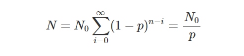
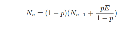
The recording timeline contains points in time at which information is stored in some kind of memory, typically when the data entered the database. This is very useful from a logging and later maintenance perspective. With it you can keep track of how quickly your database is growing on a per object basis, or revert to previous states of the database, perhaps after an erroneous load. It could have been the case that I sent all the price cuts for Black Friday into the production database but associated with the wrong products due to a faulty join.

In literature there are a couple of other names: Inscription time [Johnston] and Load date [Data Vault]. A very poor synonym I’ve seen used is Transaction time, which should be reserved for the assertion timeline alone.

The Structuring Timeline

The structuring timeline contains the point in time at which the information had a certain structure and constraints. Yes, structure and constraints change over time too. This process is referred to as schema versioning in literature, but few mention keeping a named time line for tracking when structural changes happened. If someone comes asking why there were no price cuts for Black Friday last year, you can safely assure them that ‘price cut’ was not part of your information structure at the time.

The only other name I have seen is Schema Versioning Time, but it has a too technical ring to it, in my opinion.

Unnamed Timelines

Unnamed timelines are all the points in time that do not fall within any of your named timelines. There will be values in your database that are of a time type, but that are not immediately put onto named timelines, even if the attributes themselves are named. These may be assembled onto timelines for ad-hoc purposes or they may just be used as any other descriptive attribute. A typical example would be the point of time the receipt for the stuff I bought on Black Friday was printed. You are not likely to name the timeline on which birth dates occur either.

In literature there are a couple of other names: User defined time [Snodgrass] and Happening time [Anchor]. Again, I’ve seen Transaction time used for unnamed times when the timepoint represents some event in which a transaction took place. Again, an unfortunate confusion of terminology.

Time Tracking Scope

Before implementing time in your database, you need to consider which of the timelines above and possibly others you will need, since they need to be separable in your database, possibly as different columns in the same or adjoined tables. Along with that you will also need to determine your time tracking scope. For example, is it sufficient to track changes to any part of an address or do you need to track changes of the individual parts of an address?

If tracking any change is sufficient, you can use a single point in time for the entire address. Essentially, you will be viewing a changed address, regardless of which part changed, as a new address. If you track the individual parts you will need several points in time, one for the street, one for the postal code, one for the state, and so on. In this case the same address can have different postal codes over time.

The latter approach, tracking time for every single object (attribute and relationship) can be achieved through modeling in the sixth normal form, henceforth 6NF. With it change is visible without having to make comparisons with previous rows and no data is duplicated when only a part of something is changing.

Even if you do not go as far as 6NF your time tracking scope has to be decided, since the amount of timepoints you will store depend on it. Unfortunately, in many of the source systems I regularly fetch data from, there is usually just one column named “modified date” which is documentary. In other words you can only tell something has changed and when, but not exactly what or what came before it. In these situations you can, with a proper data warehouse, provide the history the sources lost.

Orthogonality

If you have an implementation that keeps track of both appearance and assertion timepoints, this is usually referred to as a bi-temporal implementation. The reason is that events on the appearance timeline are in a sense orthogonal to events on the assertion timeline. It is possible for the same value to appear and to be asserted simultaneously, but also at different times, so a single timepoint is not sufficient to describe both events. Furthermore, what value appears may be retroactively corrected by a later assertion. When a value appears may be also modified by an assertion. Keeping both of these on the same timeline, if you think of it as storing the date and time in a single column in a table, would cause collisions and ambiguities.

When appearances and assertions are easy to tell apart, using two different timepoints to describe these may be complex but straightforward. Problems usually arise when you are faced with a different value but nobody can tell whether it is a correction of the existing value or supposed to replace it from some point in time. This may lead to corrupt data if the wrong assumptions are made. Another issue is the fact that if you want a bi-temporal implementation with both appearance and assertion timelines treated as primary, a single table with a single primary key cannot guarantee temporal integrity. This requires careful modeling, and only a few modeling techniques have this as a “built-in” feature.

Proxying

Some of the most confusing aspects of time in databases come from the use of proxying, whether deliberate or unknowingly. If we assume that I have decided to keep track of appearance, assertion, recording, and structuring timelines in my database, with 6NF time tracking scope, then I am very much all set for anything thrown at me from a querying perspective. However, that is under the assumption that all of those timepoints will be available to me when I put data into my database.

Sadly, this is often not the case. This is true both for operational systems and data warehouses. Getting information like [Using the Megastore structure as of January 5th (The database recorded on Monday 10:12:42 that ‘The manager asserted with 95% certainty on Monday at 09:15 that “The price cut will be 25% starting at midnight on Black Friday”‘)], actually never happens, yet. We do get some of the information some of the time though.

If we are in control of the database, we will always know when data is entering it. This opens up an opportunity. In the case that we do not know the assertion timepoint, say we only get “The price cut will be 25% starting at midnight on Black Friday”, we can approximate it with the recording timepoint. In this example that means missing the mark by almost an hour. As unfortunate as this is, sometimes it is the only option.

Somewhat more dangerous, but also doable, is approximating appearance timepoints with recording timepoints. Let’s say we only get “The price cut will be 25%” and we approximate it with the recording timepoint we will be dropping the price several days too early. Since recording timepoints always “happen” in the present when they come into existence, take utmost care when using it as an approximation for appearance timepoints. Still, this may sometimes also be the only option available.

Here within lies the big fallacy though. When enough approximations have been done, the different timelines become hard to distinguish, and it seems like you can use these timepoints interchangeably. This is not the case. You should always strive to get hold of the times when they are available and if proxying is necessary, and only as a last resort, then structure your loading intervals accordingly, to minimise the damage done.

Comparing Data Vault and Anchor

So far we have talked about time in databases from a theoretical perspective. There are two modeling techniques I would like to take a practical look at, taking diametrically different approaches to which timelines serve what purposes. The two techniques Anchor modeling and Data Vault are related, both being forms of Ensemble modeling, but still have many differences.

Anchor modeling utilises 6NF to provide as granular time tracking scope as possible. It designates the appearance and assertion timelines as primary for both attributes and relationships (called ties) around a concept (called anchor), while the recording timeline is documentary. Ties are attribute-like since they have a primary timeline and in that they have no identity of their own, making tie-to-tie and tie-to-attribute connections impossible, and tie-to-anchors the only option. Anchor also maintains separate metadata for the information structure in which structuring time is primary. By treating appearance and assertion timelines as primary, the database engine will ensure bi-temporal integrity. However, that needs both to be present and have functionally adequate approximations when necessary. Anchor also makes the assumption that values are exhaustive, such that an existing value cannot become NULL, and must instead be explicitly marked as “Unknown”. There no NULL values in an Anchor model.

Data Vault is similar to Anchor, but is not 6NF and instead groups attributes together (called satellites) around a concept (called hub). A single point of time is used to track all changes within a satellite, regardless of which particular attribute changed. The big difference is that Data Vault uses the recording timeline as primary for satellites. Relationships (called links) have no primary, but include a recording timepoint as documentary. Links are hub-like since they lack a primary, and can therefore have their own identities. Theoretically link-to-link and link-to-satellite connections then become possible. The implication is that relationships that change over time must be managed through other connected objects. Figuring out that some change occurred requires you to look outside of the link. Links are also, opposed to ties, always many to many, so any additional constraints have to be managed by the application layer. If appearance and assertion timelines are present in satellites or elsewhere pertain to links, they are always documentary. I do not believe Data Vault has a notion of a structuring timeline in its standard.

The advantage of Anchor is that you do not have to worry about temporal integrity after the data has entered the database. Integrity is also practically a requirement if you want to use the technique outside of data warehousing. Anchor was designed to be a general modeling technique and it is applied in several operational systems. The downside is that you need trustworthy timepoints, which can require a lot of effort and digging in the sources. Values in a source that once existed and suddenly are NULL could pose a problem if they are indeed suddenly “Unknown” and your data type does not support it to be explicitly specified. This has, in my experience, very rarely happened, and almost always the NULL means ‘deleted’, as in asserting the statement as false, which is a different thing and handled without problems. Analysts find it easy to work directly with Anchor models, thanks to it being able to serve data as it appears at or as it was asserted at without any additional work than finding the correct bitemporal time slice.

The advantage of Data Vault is that you do not have to worry at all about temporal integrity at load time. For auditing purposes, it will reproduce inconsistencies in the sources perfectly, so if you need to provide auditing and validation reports it is an excellent choice. Since Data Vault focuses specifically on data warehousing, it is also less restricted in its choice of primary timelines. However, using the recording timeline, the temporal integrity of the now documentary appearance and assertion timelines will likely have to be taken care of later. I do believe that if any business users are going to be using the data, this must be done at some point. Pushing constraints on links to the application layer has advantages if you, for example, want to prevent bigamous weddings for Christians, but allow polygamy for Mormons. The downside is that keeping consistency in a link requires more work than for a tie. In the end about the same amount of work will likely have to be done both in Anchor and Data Vault, but with additional layers in the latter. Looking at Data Vault and its choice of recording time as primary it looks like an excellent choice for a persistent staging layer, with the usually recommended Dimensional model on top as the presentable part of the data warehouse.

In my opinion both are valid options. If you like many layers, using different modeling techniques, distributing a fixed total amount of work over them, then Data Vault is a good choice. If you do not want layers, and stick to a single modeling technique, doing a fixed total amount of work for that single layer, then Anchor is a good choice. Both have been proven in practice, also for Big Data, but Data Vault has many more implementations to date.

Imprecision and Uncertainty

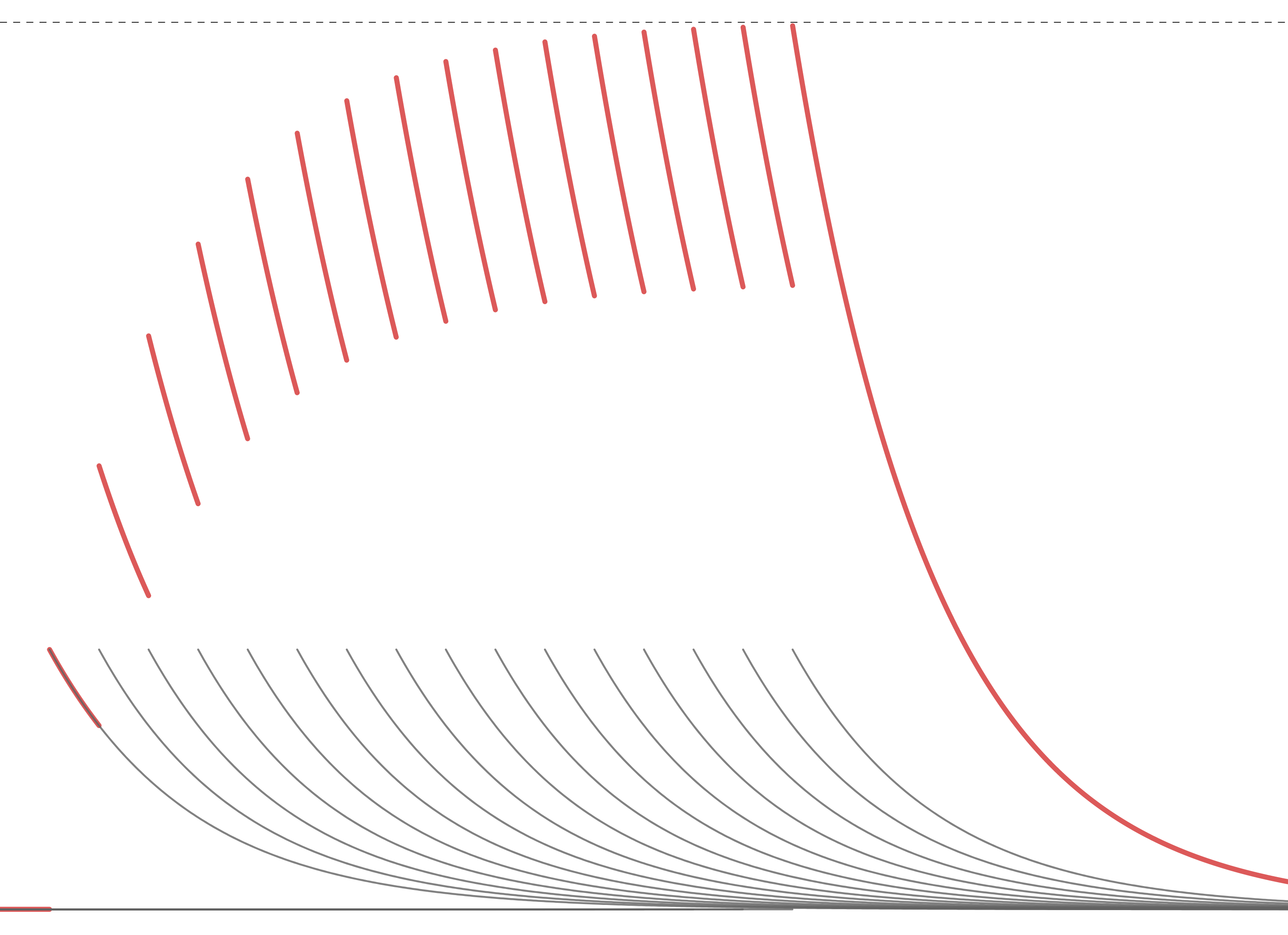
Going forward I am doing active research on transitional modeling, in which two other aspects of time is also considered. First there is imprecision. There is no way to measure time with perfect accuracy, so all timepoints are imprecise to some degree. In an atomic clock this imprecision is minuscule, but not insignificant. Regardless, there are events whose boundaries are hard to determine. Like when I got married. When exactly did that happen? Was it the moment I said “I do”? If it is, then my wife didn’t get married at the same point in time as me. By using fuzzy data types, intervals, or margins of error, we can actually express imprecision in databases. There are open questions on how to address the total ordering if we allow imprecise points of time in our primary timelines. Is it possible to maintain temporal integrity with imprecise values, or will we have to treat everything as documentary, and later apply some heuristics with best guesses?

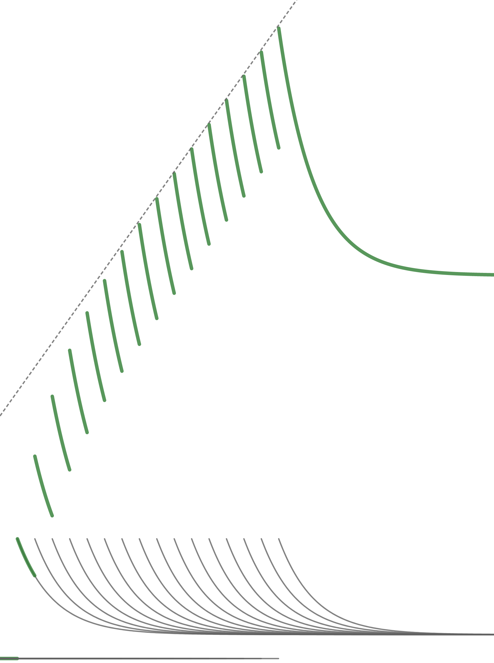
The other aspect of time is uncertainty, which is not the same thing as imprecision. Certainty is a subjective measure, in which a statement is assessed with a “probability to be true”, loosely speaking. Using certainty it is actually possible to assert that you are certain of the opposite of a statement. This takes away a hard problem of storing ‘opposite values’ in a database by instead storing a negative certainty. Taking my marriage, if I look at “Lars was married on the 19th of June 2004” I can assert with 100% certainty that it is true, even if the time is imprecise enough to pin it down to a whole day. Looking at “Lars was married between 15:00 and 16:00 on the 19th of June 2004” I may actually be less certain, and assert it with 50% certainty, since I don’t exactly remember if it was one hour earlier or not. There are some open questions on when you contradict yourself if values are imprecise and you make several (vague) assertions. If values are precise, there is an exact formula by which you can calculate exactly when you contradict yourself.

Conclusions

Hopefully I have not made time all too confusing compared to the post of Christian that inspired me. I do believe that time in databases is a complex matter, but that should be digestible for everyone, given that we can put ourselves on some common ground. All the different terminology and poor implementations out there definitely does not help.

It’s time to treat time more seriously.

Representing Large Networks by HIERARCHYID Chunks

If you recall, I wrote about “Polymorphic Graph Queries” a while ago. This exemplified the use of HIERARCHYID to represent the topology of a small computer network. As it turns out, there is a case in which the HIERARCHYID approach will explode in both numbers and size, making them an unwieldy choice, and it’s commonly seen in large networks. There is however a way to work around that issue. As far as I can tell, the graph tables in SQL Server still do not support polymorphic queries, so this workaround should be valuable.

Assume that we have a reasonably large computer network, with say a million or more devices. Representing the entire topology of the network efficiently turns out to require a combination of HIERARCHYID and traditional relational tables. HIERARCHYID performs well all the way down from locations, through enclosures, devices, and ports or antennas to the actual communication media (fiber, ethernet, wireless). Because of the large number of things connected to this layer, this is where they become unwieldy and explode in numbers. HIERARCHYID does not work well when you have intermediate layers with comparatively massive amounts of connections. Such a scenario could easily bring you into needing billions of HIEARCHYID:s. Storage skyrockets and performance goes down the drain.

Instead, by having a traditional many-to-many table represent such layers, in which different HIERARCHYID:s are related to each other, it is possible to get the best of both worlds and achieve the ability do sub second searches through the topology. Let’s call the structure (UID, HIERARCHYID) a chunk, where the UID can typically be an integer. The relational table can then be as simple as (UID, UID) indicating that two chunks are connected, only requiring as many rows as there are connections. Polymorphic queries now need to take this into account, by first finding a number of candidate chunks, then join these through the relational table to discard ones that are not connected, which yields the final result.

A similar recursive query used for testing a relational parent-child hierarchy of the same network had to be stopped after having run for several hours. The benefit of HIERARHYID is substantial, but only if you take special care of layers with high connectivity. For small uncomplicated hierarchies, like employees and managers at a company, a traditional representation with less complexity is likely sufficient. Some alternatives can be found in “Hierarchical Data in SQL” by Ben Brumm.

PostgreSQL 12 and Editing en masse

Thanks to the great work of Juan-José van der Linden, a fresh PostgreSQL generator is taking form in the test version. He also added data type conversions between the available target databases and lists with suggested datatypes that simplify entering types in the interface. Before this work was added we decided to release version 0.99.6.3, so that it will remain stable. This minor version, albeit while in test, has been used in production for quite some time at our clients.

PostgreSQL generation in the test version.

On top of that we have also modularized the code, fixed a few bugs, and implemented some long standing pull requests. A so far rather rudimentary, but useful, editor has been added. This allows editing of an anchor and all of its attributes in the same view. Bring it up by pressing Shift+E on your keyboard while hovering over the desired anchor.

Editing en masse with some newly created attributes.

Tinker Take Two

I bought another Raspberry Pi 4B to replace an old 3B+ that did not want to play along any more. It had been acting as a web server, so it will need less software than the job scheduling server. The old server had been running Raspbian, but I am so satisfied with Alpine that I decided to switch, so I followed the first tinkering guide, but only installed:

apk add nano nodejs npm screen sudo

I only need nodejs, since that is what is used for the web server. After that I wanted to harden the system, but it turns out that ufw has moved to the edge community repository. In order to activate it edit /etc/apk/repositories.

nano /etc/apk/repositories

Add a tag named @community for it, and if you like me want the kakoune text editor then also add @testing, making the contents look as follows.

#/media/mmcblk0p1/apks
http://ftp.acc.umu.se/mirror/alpinelinux.org/v3.12/main
#http://ftp.acc.umu.se/mirror/alpinelinux.org/v3.12/community
#http://ftp.acc.umu.se/mirror/alpinelinux.org/edge/main
@community http://ftp.acc.umu.se/mirror/alpinelinux.org/edge/community
@testing http://ftp.acc.umu.se/mirror/alpinelinux.org/edge/testing

Update to get the new package lists, then add and configure ufw.

apk update
apk add ufw@community
rc-update add ufw default 
ufw allow 2222 
ufw limit 2222/tcp
ufw allow 80
ufw allow 443

After that I followed the guide to disallow root login, enable ufw, and reboot, with one exception. When editing sshd_config I also changed to a non-standard port to get rid of most script kiddie attempts to hack the server. Find the line with:

#Port 22

and uncomment and change this to a port of your liking, for example:

Port 2222

Trust by Certificate

After logging in as the non-root user I created when following the guide, I can still switch to root by using su. I need to add certbot, that keeps the certificate of the server up to date and restore the contents of the www folder.

su
apk add certbot@community
cd /var
mount -t cifs //nas/backup /mnt -o username=myusr,password=mypwd
tar xvzf /mnt/www.tar.gz

Now when that is in place it’s time to update the certificates.

certbot certonly

Since I haven’t started any web servers yet, it’s safe to select option 1 and let certbot spin up it’s own. After entering the necessary information (you probably want to say “No” to releasing your email address to third parties), it’s time to schedule certbot to run daily. It will renew any certificates that are about to expire in the next 30 days.

cd /etc/periodic/daily
nano certbot.sh

The contents of this file should be (note that Alpine uses ash and not bash):

!/bin/ash
/usr/bin/certbot renew --quiet

After that, make that file executable.

chmod +x certbot.sh

With that in place I can start my own web server. It’s an extremely simple static server. The Node.js code uses the express framework and is found in a script named static.js with the following contents.

var express = require('express');
var server = express();
server.use('/', express.static('static'));
server.listen(80);

The HTML files reside in a subdirectory named “static”. For now I run the server in a screen, but will likely add a startup script at some point.

Superuser Do and Terminal Multiplexing

Since the server will listen on the default port 80 I need sudo privileges to start it. The recommended way is to let members of the wheel group use sudo. Depending on what you picked for a username, exemplified by “myusr” here, run the following.

echo '%wheel ALL=(ALL) ALL' > /etc/sudoers.d/wheel
adduser myusr wheel
exit
whoami
exit

The exit will return you to your normal user, from being root since “su” earlier. The second exit will end your session and you will have to log in again, in order for the “wheel” to stick.

screen
sudo node static.js

This will run the server in the foreground, so to detach the screen without cancelling the running command, press “Ctrl+a” followed by “d”. To check which screens are running you can list them.

screen -ls

This will list all screens:

There is a screen on:
3428.pts-0.www (Detached)
1 Socket in /tmp/uscreens/S-myusr.

In order to reattach to one of the listed screens, you do so by it’s session number.

screen -r 3428

Encrypted Backup to the Cloud

I will be hosting some things that I want to have a backup of, and this web server will not be running on a separate subnet, so my NAS is not accessible. I’ll therefore be backing up to OneDrive (in the cloud) using rclone. You will need access to rclone on a computer with a regular web browser to complete these steps. For this, I download rclone on my Windows PC. I will elevate privileges using su first.

su
apk add curl bash unzip
curl https://rclone.org/install.sh | bash

With rclone installed it is time to set it up for access to OneDrive.

rclone config

Select “New Remote”, and I named mine “onedrive”, then choose the number corresponding to Microsoft OneDrive. Leave client_id and client_secret as blanks (default values). Select “No” to advanced config and again “No” to auto config. Here is where you will need to follow the instructions and move to your computer with the web browser to get an access_token. Once this is pasted back into the config dialogue next select the option for “OneDrive Personal”. Select the drive it finds and confirm it is the right one and confirm again to finish the setup. Quit the config using “q” and test that the remote is working properly.

rclone ls onedrive:

Provided that worked, it is now time to enable encryption of the data we will be storing on OneDrive. Start the config again.

rclone config

Select “New Remote” and give this a different name, in my case “encrypted”, then choose the number corresponding to Encrypt/Decrypt. You will then need to decide on a path to where the encrypted data will reside. I chose “onedrive:encrypted” so that it will end up in a folder named “encrypted” on my OneDrive. I then selected to “Encrypt filenames” and “Encrypt directory names”. Then I provide my own password, since this Raspberry Pi will surely not last forever. I won’t be remembering salt, so I opted to leave it blank. Choose “No” to advanced config and “Yes” to finish the setup.

With that in place I will create a script that performs the backup, placed in the folder that I want to backup. I am going to run this manually and only when I’ve been editing any of the files I need to backup.

nano backup.sh

This file will have the following contents.

!/bin/sh
/usr/bin/rclone --links --filter "- node_modules/**" sync . encrypted:

It will filter out the nodejs modules, since they can and will be redownloaded when you run node anyway. After testing this script I can see something like the following on my OneDrive in the encrypted folder.

Prerequisites for Node.js Development

Since I moved from a 32-bit to a 64-bit operating system, some npm modules may be built for the wrong architecture. I will clean out and refresh all module dependencies using the following. There are lots of modules in my system, since it actually does more than just run a static web server, like being the foundation for Rita (our robotic intelligent telephone agent). Some modules may need to be built, which is why we need to add the necessary software to do so.

rm -Rf node_modules
apk add --virtual build-dependencies build-base gcc wget git
npm install
npm audit fix

For better editing of actual code (than nano) I will be using kakoune.

apk add kakoune@testing

Now, if you will be running this from Windows I highly recommend using a terminal with true color capabilities, such as Alacritty. Colors will otherwise not look as nice as in the screenshot below (using the zenburn colorscheme).

I believe that is all, and this server has everything it needs now. Those paying particular attention to the code in the screenshot will notice that the underlying SQLite database is Anchor modeled.

I am writing this guides mostly for my own benefit as something to lean on the next time one of my servers call it quits, but they could very well prove useful for someone else in the same situation.